Module 9 - Test bank

This bank has four sections. The first two contain 5 questions each about interpreting field-level data and deciding what we can learn from it. Sections 3 and 4 contain worked examples of the tasks you should be able to carry out with harvest and satellite data. In each section, we work through a real field and a field with simulated harvest data.

The module test will contain two questions from the first two sections and two tasks like those in Sections 3 and 4. You will answer the first two questions on Canvas without help from AI. You can use AI to help with the last two. Those tasks will use a field you have not seen before, so focus on understanding what each step does. You will need to adapt the code to the new file and its column names.

The data

The worked examples in Sections 3 and 4 use a barley field and a wheat field. The fields in this bank are all between about 115 and 155 acres, in and around the RM of Blaine Lake and Corman Park, north of Saskatoon.

• example_wheat.csv – 123 acres of spring wheat, 24,637 readings.
• example_barley.csv – 152 acres of barley, 37,957 readings. This file uses different column names from the wheat file.
• example_barley_ndvi.csv – NDVI for the barley field, one row per pixel per date.
• example_wheat_boundary.geojson / example_barley_boundary.geojson – the field boundaries.
• example_wheat_wetlands.geojson – the sloughs inside the wheat quarter.
• example_wheat_ndvi.zip – Sentinel-2 NDVI for the wheat field, one 10 m raster per week of the 2026 season, named wheat_ndvi_2026-W<week>.tif. Unzip it into your data/ folder.

The wheat harvest file holds one row per second, with the columns iso_time, longitude, latitude, yield (bu/ac), moisture, speed_mph, width_ft, elevation, pass_num, field, crop and variety.

The barley file uses different column names. In example_barley.csv, used in Section 3, yield is called yield_bu_ac, cutting width is swath_ft, elevation is elev_ft and moisture is moisture_pct.

---

Section 1 — What one field can tell you

Question 1

A yield monitor is incorrectly calibrated, so every reading is 10% too high.

(a) How does this affect the field average?

(b) Would the map still be useful for finding the better and poorer parts of the field? Explain.

(c) Would taking more readings with the same calibration solve the problem?

Answer

(a) The average is also 10% too high.

(b) Yes. Every reading is 10% too high, so the better parts of the field still appear better and the poorer parts still appear poorer. The map can show that pattern even though the yield values themselves are wrong.

(c) No. The additional readings would have the same calibration error. We would need to check the monitor against something independent, such as grain loads weighed on a scale.

Question 2

A farmer points to an empty cell between two passes on a 10 m yield map and says, “Nothing grew there.”

(a) What else could explain the empty cell?

(b) Is an empty cell the same as a cell with a recorded yield of zero? Explain.

Answer

(a) The grid averages readings whose recorded positions fall inside each cell. A cell between pass centres can contain no recorded point even though the header cut crop there. It may also be empty because readings were removed during cleaning. The map alone does not show that nothing grew.

(b) An empty cell has no usable yield measurement assigned to it. A recorded zero is a value reported by the monitor, which still needs interpretation: for example, the machine may have been running without grain flowing. We should therefore keep missing readings separate from recorded zeros.

Question 3

An agronomist uses one season of data from a 140-acre canola field. Late-July NDVI has a correlation of 0.45 with yield. She holds back some cells to test her model and gets a prediction error of 2.9 bu/ac, compared with a yield standard deviation of 3.2. She concludes: “We can use satellite imagery to forecast canola yields across the district before harvest.”

(a) Why doesn’t her test tell us whether the model will work across the district?

(b) She has 3,600 cells. Would having 36,000 cells from this same field solve the problem? Explain.

(c) What additional data would you want, and which observations would you hold back to test the district forecast?

Answer

(a) The hold-out cells come from the same field in the same year. They share one soil, one variety, one seeding date and one season’s weather with the cells the model was fitted on. So the test shows the model predicts unseen parts of this field, which is a real result but a narrow one. A district forecast asks it to predict fields it has never seen, and no such field appears anywhere in the data.

(b) More cells give us more detail about this field, but do not add other fields or seasons. Every new cell still carries the same soil, the same season and the same management, so none of them tells the model anything about a field that differs in those respects. We still would not know how the model performs under different growing conditions.

(c) Many fields, across several seasons, spanning the range of soils, varieties and weather the forecast is meant to cover. The hold-out would have to be whole fields and whole years – fit on some fields, test on fields the model has never seen – because that is the question being asked. Holding out cells cannot test it no matter how many fields are in the data.

Question 4

You can map a 140-acre field using 10 m, 20 m or 50 m cells. Which would you choose for each of the following, and why?

(a) Showing the farmer the main yield patterns in the field.

(b) Choosing where to take soil samples in a patch that repeatedly yields poorly.

(c) Preparing a variable-rate seeding prescription for a drill with 40-foot sections.

(d) Comparing the field’s average yield with last year’s average.

Answer

There is more than one reasonable answer to each part. Explain your choice in terms of what the map will be used for, what the equipment can do, or how precisely you need to locate a patch. The answers below are examples.

(a) 20 m. It is fine enough to show the pattern that matters – the low ground, the headlands, the good middle – without the empty stripes between combine passes that a 10 m map carries. This makes the main patterns easier to see.

(b) 10 m, or the raw readings. Here the aim is to locate something precisely enough to go and stand on it, and a 20 m cell averages over a quarter of an acre. The gaps between passes are a nuisance rather than a problem, because you are looking for where a patch is, not producing a continuous surface.

(c) 50 m, or something close to it. The drill cannot act on anything finer than its own working width, so a prescription at 10 m asks the machine to change rate several times within one pass, which it cannot do and would not help if it could. The resolution should be matched to what the equipment can execute, not to what the data can resolve.

(d) Resolution is almost irrelevant – the answer is a single number, and the field average comes out much the same at any cell size. What matters far more is that both years are computed the same way, on the same area, with the same cleaning rules. A difference in method between the two years would swamp any difference from resolution.

Other choices can also be justified. For example, you might choose 10 m for (a) to show the farmer more detail, or 20 m for (c) and then smooth the prescription. What matters is explaining why the resolution suits the task.

Question 5

A consultant has built a yield model using satellite images from 400 fields in southern Saskatchewan over four seasons. It predicts reasonably well on fields that were left out when fitting the model. A client wants to use it on three quarters they have bought in Alberta’s Peace River region.

(a) What gives you some confidence that the model might work there?

(b) What makes you cautious about using it there?

(c) What would you recommend to the client, and how could they check whether the predictions are useful?

Answer

(a) The model was tested the right way – held out at the level of whole fields, across four seasons and 400 fields, so it has seen genuine variety in soil, weather and management rather than one field’s worth. That is a much stronger basis than a single-field model, and the relationship it uses – greenness during grain fill tracks yield – is a biological one rather than an accident of one place.

(b) The Peace River region is outside the range of everything the model was fitted on: different soils, a shorter and cooler season, longer summer days, different varieties and different typical yields. Asking the model about it is extrapolation, and a model gives an answer outside its range just as confidently as inside it. Nothing in the hold-out test measured performance there, because nothing like it was in the data.

(c) Tell them the model is well built for southern Saskatchewan and is being asked a question outside what it has seen, so its predictions for those quarters should be treated as untested rather than as wrong. Then ask them to run it on the new quarters alongside whatever they actually harvest, for a season or two, and compare. Comparing predictions with actual harvests would give them evidence about how well the model works on those fields.

Section 2 — Judgement and interpretation

Question 1

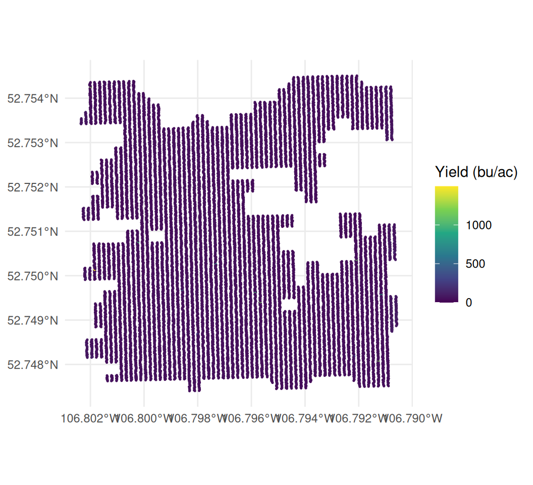
You read in a yield file and make the map below.

Figure 2.1: A student’s first map of a canola field.

(a) Why is almost the whole field the same colour? Give one line of R that would help check your explanation.

(b) How could you make the yield differences easier to see? Give two options and explain what each changes or leaves out.

(c) The legend reaches nearly 1,500 bu/ac. What should you investigate in the data before improving the plot?

Answer

(a) A handful of extreme readings are stretching the colour scale. The legend runs to almost 1,500 bu/ac while the field is actually around 42, so ordinary yields occupy a very small part of the scale and appear almost the same colour.

summary(canola_q1$yield)
quantile(canola_q1$yield, c(0.5, 0.99, 1))

> summary(canola_q1$yield)
   Min. 1st Qu.  Median    Mean 3rd Qu.    Max. 
   0.00   37.47   41.97   42.81   46.46 1497.44 
> quantile(canola_q1$yield, c(0.5, 0.99, 1))
    50%     99%    100% 
  41.97   70.88 1497.44 

The 99th percentile is about 71 bu/ac and the maximum is 1,497 – more than twenty times it. A small number of extreme readings therefore determines most of the colour scale.

(b) Either drop the impossible readings before plotting, which is right because they are not measurements of a crop, but means you can no longer see where in the field they occurred; or keep them and fix the scale with limits plus oob = scales::squish, which keeps every point on the map but stops distinguishing between anything above the cut-off. The second is better when the question is where the bad readings are – and here that matters, because they are not scattered at random.

(c) That the file has not been cleaned. No canola crop yields 1,497 bu/ac, so at least one reading in the file is not a measurement of grain. Before any map is worth looking at, those readings need finding and flagging. The plot has helped identify a problem that needs checking in the data.

Question 2

A canola field is shown below at four cell sizes, after the impossible readings and the partial-width passes have been removed. Each cell is the average of the readings that fall inside it.

Figure 2.2: A canola field averaged into 10, 20, 40 and 80 m cells.

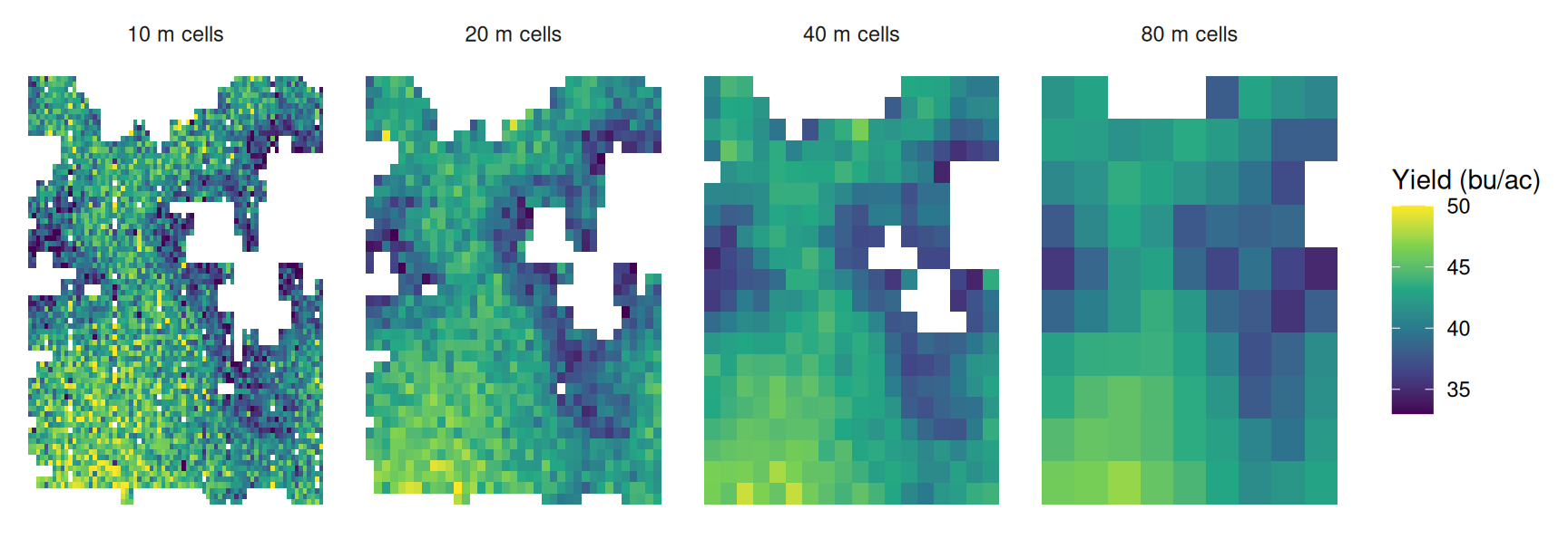
The four maps come from the same readings. Their summary statistics are:

Cell size	Cells	Mean	SD	Lowest cell	Highest cell
10 m	4,279	41.70	4.01	22.3	60.7
20 m	1,162	41.63	3.03	31.4	50.2
40 m	315	41.58	2.83	34.5	48.6
80 m	85	41.29	2.75	34.8	47.2

(a) The mean hardly changes but the standard deviation falls by a third. Explain why.

(b) At 10 m the worst cell is 22.3 bu/ac and at 80 m it is 34.8. Has the bad ground improved? What happened to it?

(c) Look at the two white holes in the field. Describe what happens to them from left to right, and explain why.

(d) A farmer wants to find spots worth investigating on foot. Another wants a single figure for a whole-field fertiliser rate. Which map suits each, and why?

Answer

(a) The mean is the average of the same readings however they are grouped, so it barely moves. The standard deviation falls because a single reading carries all the second-to-second noise of the monitor, while an 80 m cell averages several hundred readings and most of that noise cancels. The spread that disappears is mostly measurement error rather than real variation in the field.

(b) No. The 22.3 cell was a small patch where a handful of noisy low readings happened to land together. At 80 m it has been averaged in with the better ground around it, so the low value is diluted rather than removed. The extremes at both ends shrink for the same reason – which is why the range narrows from 22-61 to 35-47 even though the field is unchanged.

(c) They are the sloughs, where nothing was harvested and so there are no readings. At 10 m they are sharply outlined. As the cells grow, a cell that straddles the edge of a slough picks up the harvested readings next to it and is drawn as ordinary ground, so the holes shrink and blur. By 80 m they have nearly closed up. Coarsening the grid does not just smooth the values, it moves the boundary of where the field is.

(d) The farmer walking the field wants 10 m or 20 m: the point is to locate small areas, and a coarse map has averaged them away. The one setting a single rate can use any of them – they all give about 41.6 – so the coarse map costs nothing and is the easier one to read. Choose the resolution based on what you need to learn from the map.

Question 3

Five years of one field are mapped below on one shared colour scale. The crop was different each year.

Figure 2.3: One field, five seasons, all on one bushels-per-acre scale.

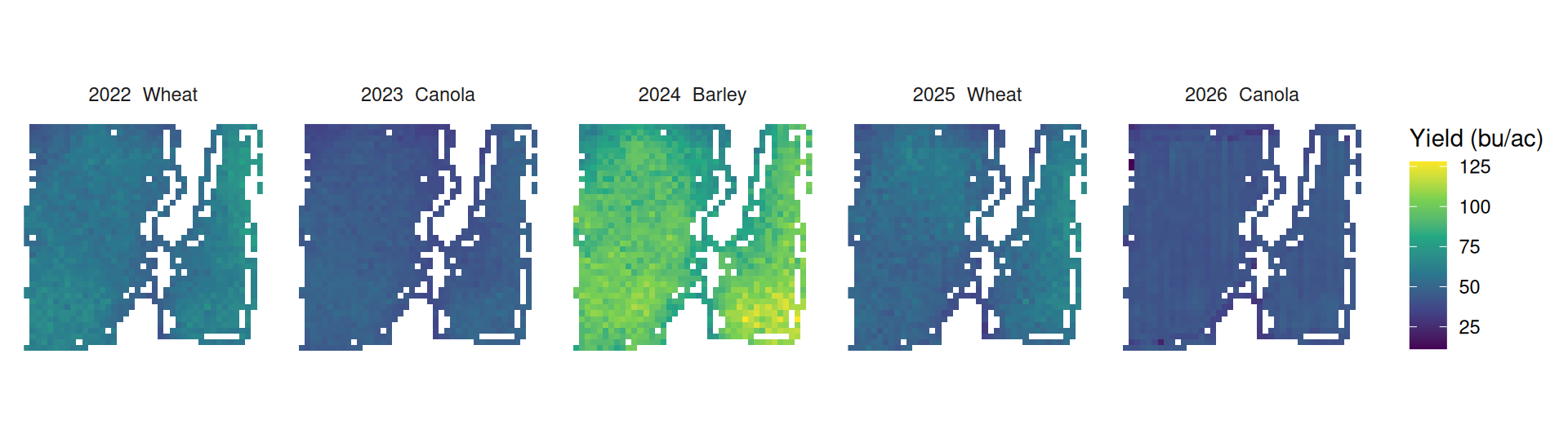
(a) 2024 is much brighter than the other four years. Does that mean 2024 was the best season on this field? Explain.

(b) Four of the five maps look nearly uniform. Is that because those fields really were uniform?

(c) A manager concludes from these maps that the field has no consistent weak areas. Why can that conclusion not be drawn from this figure?

(d) Suggest a change to the figure that would let the five years be compared, and say what your version can and cannot show.

Answer

(a) No. 2024 was barley, and barley yields far more bushels per acre than wheat or canola because the bushel is a unit of volume and the crops differ in what a bushel weighs and in how much the plant produces. Putting 92 bu/ac of barley on the same scale as 44 bu/ac of canola compares the crops, not the seasons. Whether 2024 was a good barley year can only be judged against other barley years.

(b) No. They look uniform because the scale has to stretch from the bottom of the canola years to the top of the barley year, roughly 25 to 125 bu/ac. Within-year variation on this field is a few bushels either side of the mean, which occupies only a small part of that range. The scale makes those differences difficult to see. This is similar to the colour-scale problem caused by an extreme reading, although here the wide range comes from comparing different crops.

(c) Because the figure cannot show weak areas either way. A map that renders almost everything in one colour is not evidence of uniformity – it is evidence that the scale is wrong for the question. We need a scale that shows the differences within each year before deciding whether the same areas repeatedly yield poorly.

(d) Convert each year to a within-year measure before mapping – a percentile rank, a z-score, or yield as a share of that year’s field mean – and give every panel the same scale in those units. Then a cell that is poor relative to its own year reads the same whatever crop was grown.

What that version shows is the spatial pattern: which parts of the field are consistently at the bottom. What it deliberately throws away is the level – every year is rescaled to look equally variable, so a year where the whole field did badly is indistinguishable from a good one. If the question is “which ground is weak”, that is the right trade. If it is “how did the field do”, it is the wrong one.

Question 4

A consultant defines the field’s poor ground as the worst 20% of cells and maps it at three cell sizes.

Figure 2.4: The bottom 20% of cells in a canola field, at three cell sizes.

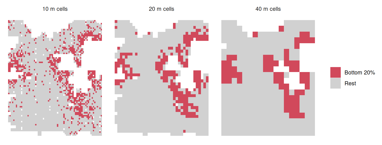
Comparing the 10 m and 40 m maps cell by cell: of the ground flagged at 10 m, 57% is still flagged at 40 m and 43% is not, and the 40 m map flags ground the 10 m map passed over.

(a) All three maps flag exactly a fifth of the cells. Why, then, do they disagree about which ground is poor?

(b) At 10 m the poor cells are scattered across the field; at 40 m they form a band around the sloughs. Which is the better description of where this field is weak?

(c) The consultant is choosing where to pull soil cores. Does the disagreement matter? What about if they were costing out a drainage project?

(d) The rule “flag the bottom 20%” always flags 20%. What would a rule need instead for the answer to mean something?

Answer

(a) Because a 10 m cell holds only a handful of readings, so its average still carries a lot of the monitor’s noise, and a cell can fall in the bottom fifth because of a few unlucky readings rather than poor ground. A 40 m cell averages sixteen times as many readings, so noise largely cancels and what remains is mostly real. The two maps are ranking different mixtures of signal and noise, so they rank different cells last. Both maps select 20% of cells, but averaging changes which cells fall into that group.

(b) The 40 m map, for the purpose of describing where the field is weak. Weakness that is real and worth managing is caused by things with spatial extent – drainage, salinity, a knoll – and those show up as contiguous areas. A speckle of isolated 10 m cells scattered through good ground is mostly noise, and it is difficult to use those scattered cells to define a management area. The caution is that 40 m also smooths away genuinely small problem areas, so the coarse map is the better summary without being the more detailed truth.

(c) For soil cores it matters, but it is not fatal – you are sampling to learn something, the cores can be placed in the consistently flagged ground where both maps agree, and a misplaced core costs one sample. For a drainage project it matters a great deal: the decision is expensive and hard to reverse, and 43% of the flagged area changing identity with an arbitrary analysis choice means the map is not a reliable basis for it. Before an expensive decision, we would want to understand why changing cell size changes the selected area so much.

(d) It would need an absolute threshold tied to something outside the data – a yield below which the ground does not pay for the inputs it receives, for instance, so the rule can return 2% of the field or 40% or none of it. A relative rule answers “which fifth is worst” and will do so on a perfectly uniform field. An absolute rule can answer “is any of this field actually bad”, which is the question being asked.

Question 5

Three maps of the canola field, all 20 m cells, all the same yield data. Only the colour scale differs.

Figure 2.5: One gridded yield surface, three colour scales.

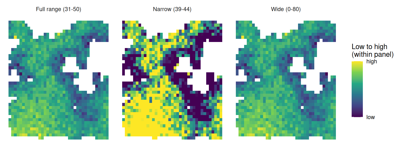
The cells run from 31.4 to 50.2 bu/ac, with a standard deviation of 3.0. Half of them lie between 39.6 and 43.8.

(a) The middle map shows large solid areas of high and low yield. Is it showing a real pattern?

(b) The right-hand map suggests a uniform field. Is that an honest summary?

(c) An agronomist selling variable-rate prescriptions puts the middle map in a sales presentation. What is misleading about it, given that nothing in the data was altered?

(d) You have to pick one of these for a report. Which, and what would you state alongside it?

Answer

(a) The areas do differ in yield – those areas genuinely are above and below the field average, and the shape matches the sloughs and the eastern strip seen in other maps. The colours, however, make the differences look larger than they are. The scale spans 39 to 44 bu/ac, so the difference between solid yellow and solid purple is about 5 bu/ac, and everything above or below the window is flattened into the same extreme colour. A reader who has not studied the legend sees a field of dramatic extremes; the data shows a field varying by a few bushels.

(b) No. In this case the scale is too wide. The scale runs from 0 to 80 while the data occupies 31 to 50, so most of the colour range is spent on yields that do not occur, and the real variation is squeezed into a narrow band of near-identical greens. There is a genuine and consistent pattern in this field, and this map conceals it. Both of the outer maps are distortions; they distort in opposite directions.

(c) The map can give the reader an exaggerated impression of how much yields differ. Someone selling variable-rate seeding needs the field to look like it has distinct zones worth treating differently, and a narrow colour window manufactures exactly that appearance from a 5 bu/ac spread. The yield values have not changed, but the narrow scale makes the differences appear more dramatic. That is why the colour scale needs to be considered when interpreting the map.

(d) The left-hand map, scaled to roughly the range of the data. Alongside it, report the size of the differences: the cells run 31 to 50 bu/ac, the standard deviation is 3.0, and half the field lies within about 4 bu/ac of the median. A reader can then judge whether a pattern that is clearly present is also large enough to act on. The map alone cannot tell us whether changing management would pay.

---

Section 3 — Cleaning and mapping a field

In this section, we will work through the steps involved in cleaning and mapping a harvest file. You should be able to:

1. Read in the data and check the number of rows and the columns it contains.
2. Check for outliers and explain which readings you would flag and why.
3. Map the raw combine data, showing each reading as a point.
4. Create a yield grid by averaging readings within cells.
5. Add the field boundary to the gridded map.
6. Summarise the field, including average yield, average moisture and an estimate of harvested area. Compare that area with the area inside the field boundary.

On the test, you will be given a harvest file and asked to carry out some of these steps. Start by looking at the file. The column names may differ from the examples below, and you will need to work out which columns contain the information you need.

The examples below work through all six steps, first with the barley field and then with the wheat field.

Example 1 — the barley field

We will start with example_barley.csv, which contains 37,957 barley harvest readings. The field boundary is in example_barley_boundary.geojson.

Steps 1 and 2: read in the file and check the yields.

library(tidyverse)

barley <- read_csv("data/example_barley.csv")
dim(barley)
summary(barley$yield_bu_ac)

> library(tidyverse)
> 
> barley <- read_csv("data/example_barley.csv")
Rows: 37957 Columns: 12
── Column specification ────────────────────────────────────────────────────────
Delimiter: ","
chr (3): field, crop, variety
dbl (9): seconds_in, yield_bu_ac, moisture_pct, speed_mph, heading_deg, elev...

ℹ Use `spec()` to retrieve the full column specification for this data.
ℹ Specify the column types or set `show_col_types = FALSE` to quiet this message.
> dim(barley)
[1] 37957    12
> summary(barley$yield_bu_ac)
   Min. 1st Qu.  Median    Mean 3rd Qu.    Max.     NAs 
    0.0    97.3   104.5   105.0   111.9 69895.6      31 

The median yield is 104.5 bu/ac, but the maximum is 69,896 bu/ac. There are also 31 rows with missing yield. The median is a believable barley yield; the maximum clearly is not. We need to look more closely at these extreme readings before using the data.

## Where does the distribution stop being plausible?
quantile(barley$yield_bu_ac, c(0.5, 0.99, 0.999, 1), na.rm = TRUE)

## Count the rows each problem affects.  Nothing in the file marks these --
## we have to go looking for them
barley |>
  summarise(
    missing  = sum(is.na(yield_bu_ac)),
    zero     = sum(yield_bu_ac == 0, na.rm = TRUE),
    over_300 = sum(yield_bu_ac > 300, na.rm = TRUE),
    partial  = sum(swath_ft < 39)
  )

> ## Where does the distribution stop being plausible?
> quantile(barley$yield_bu_ac, c(0.5, 0.99, 0.999, 1), na.rm = TRUE)
       50%        99%      99.9%       100% 
  104.4550   131.5775   193.6575 69895.6000 
> 
> ## Count the rows each problem affects.  Nothing in the file marks these --
> ## we have to go looking for them
> barley |>
+   summarise(
+     missing  = sum(is.na(yield_bu_ac)),
+     zero     = sum(yield_bu_ac == 0, na.rm = TRUE),
+     over_300 = sum(yield_bu_ac > 300, na.rm = TRUE),
+     partial  = sum(swath_ft < 39)
+   )
# A tibble: 1 × 4
  missing  zero over_300 partial
    <int> <int>    <int>   <int>
1      31   664       24    3103

Almost all the yields are much lower than the maximum: the 99th percentile is 131.6 bu/ac and the 99.9th is 193.7. The very large values therefore come from only a few rows.

Counting each problem separately shows what we are dealing with: 31 rows with no yield recorded, 664 zeros, 24 readings above 300 bu/ac, and 3,103 rows where the combine was not cutting a full header width. The last group is the largest by far, and it is the one that is easiest to miss – those yields look perfectly reasonable on their own.

## Drop what cannot be real, and keep only full-width cutting.
## A partial swath makes the monitor divide by the wrong width, so those
## readings run high even though nothing is wrong with the crop
clean <- barley |>
  filter(!is.na(yield_bu_ac), yield_bu_ac > 0, yield_bu_ac < 300, swath_ft >= 39)

nrow(barley)
nrow(clean)
nrow(barley) - nrow(clean)

> ## Drop what cannot be real, and keep only full-width cutting.
> ## A partial swath makes the monitor divide by the wrong width, so those
> ## readings run high even though nothing is wrong with the crop
> clean <- barley |>
+   filter(!is.na(yield_bu_ac), yield_bu_ac > 0, yield_bu_ac < 300, swath_ft >= 39)
> 
> nrow(barley)
[1] 37957
> nrow(clean)
[1] 34511
> nrow(barley) - nrow(clean)
[1] 3446

Step 3: map the combine readings.

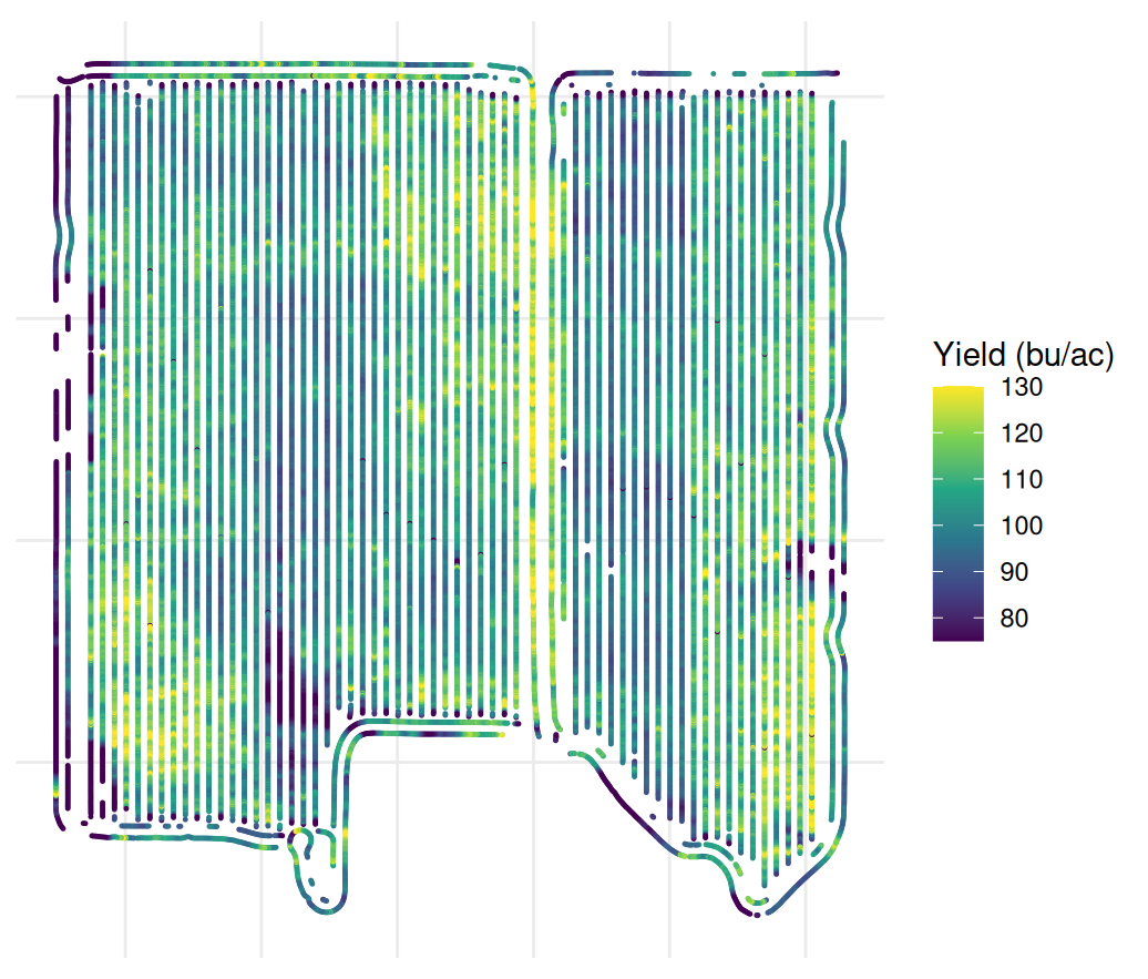
We can use the coordinates to plot one point for each reading and see the path the combine took through the field.

Figure 3.1: The barley field, cleaned combine readings.

Steps 4 and 5: average the readings into 20 m cells and add the field boundary.

As in the chapter, we first project the points into metres. We can then create a grid, average the readings in each cell and plot the result with the boundary.

library(sf)
library(terra)
library(tidyterra)

## Project to UTM 13N so the cells are a real 20 m, not 20 degrees
pts <- clean |>
  st_as_sf(coords = c("longitude", "latitude"), crs = 4326) |>
  st_transform(32613) |>
  vect()

## rasterize() is the points-to-raster inverse of extract().  Build the
## template from the points themselves and every cell lines up by construction
grid  <- rast(pts, resolution = 20)
yield_r <- rasterize(pts, grid, field = "yield_bu_ac", fun = mean)

yield_r
global(yield_r, "mean", na.rm = TRUE)

> library(sf)
> library(terra)
> library(tidyterra)

Attaching package: 'tidyterra'
The following object is masked from 'package:stats':

    filter
> 
> ## Project to UTM 13N so the cells are a real 20 m, not 20 degrees
> pts <- clean |>
+   st_as_sf(coords = c("longitude", "latitude"), crs = 4326) |>
+   st_transform(32613) |>
+   vect()
> 
> ## rasterize() is the points-to-raster inverse of extract().  Build the
> ## template from the points themselves and every cell lines up by construction
> grid  <- rast(pts, resolution = 20)
> yield_r <- rasterize(pts, grid, field = "yield_bu_ac", fun = mean)
> 
> yield_r
class       : SpatRaster
size        : 43, 40, 1  (nrow, ncol, nlyr)
resolution  : 20, 20  (x, y)
extent      : 393884.8, 394684.8, 5778910, 5779770  (xmin, xmax, ymin, ymax)
coord. ref. : WGS 84 / UTM zone 13N (EPSG:32613)
source(s)   : memory
name        :       mean
min value   :      4.305
max value   : 135.213529
> global(yield_r, "mean", na.rm = TRUE)
         mean
mean 102.5307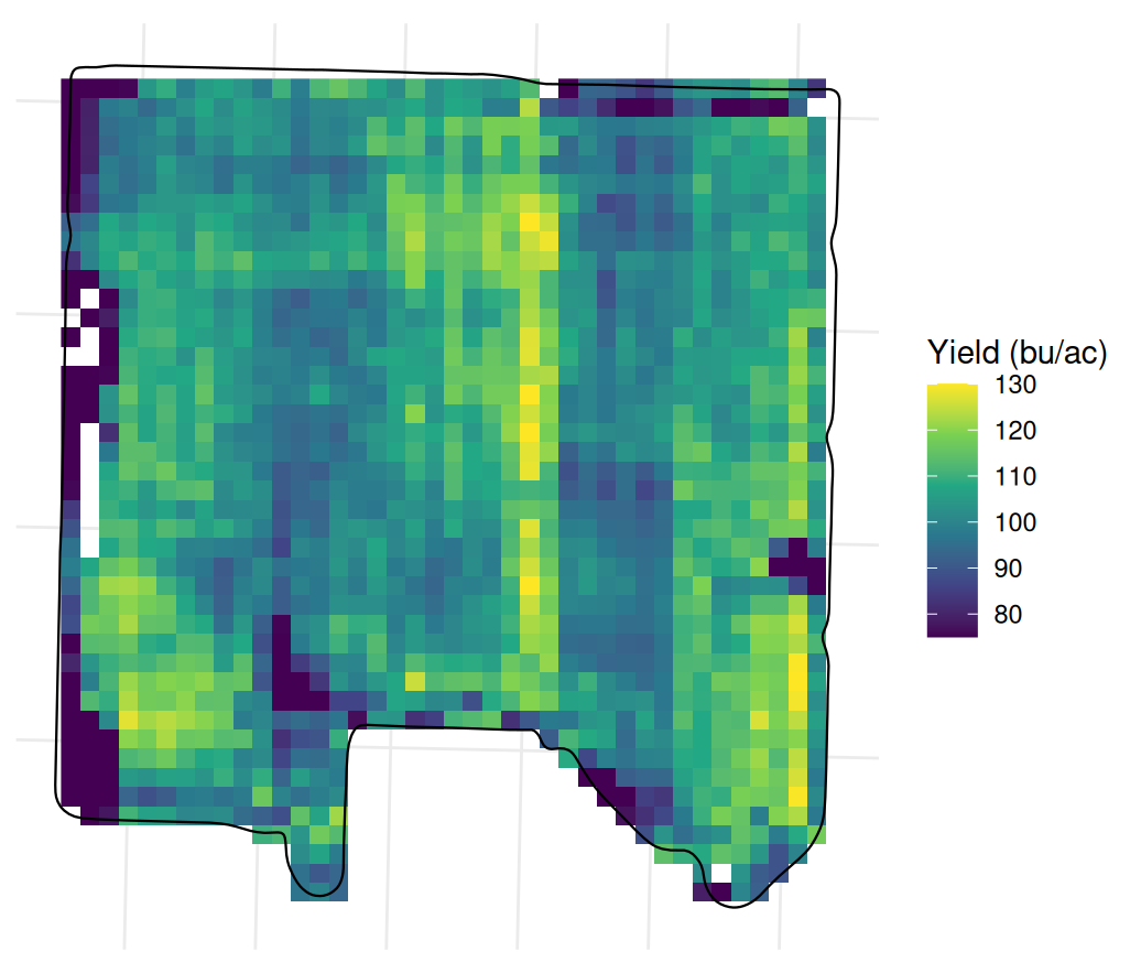

Figure 3.2: The barley field gridded to 20 m cells, with the field boundary.

Step 6: summarise the field.

## Field-level aggregates, from the cleaned readings
clean |>
  summarise(
    n            = n(),
    mean_yield   = mean(yield_bu_ac),
    median_yield = median(yield_bu_ac),
    sd_yield     = sd(yield_bu_ac),
    mean_moist   = mean(moisture_pct, na.rm = TRUE),
    mean_speed   = mean(speed_mph)
  )

## Harvested area is the number of 20 m cells that got a reading,
## 400 square metres each
n_cells <- sum(!is.na(values(yield_r)))
n_cells
n_cells * 400 / 4046.86

## The boundary says how big the field is
bnd <- st_read("data/example_barley_boundary.geojson", quiet = TRUE) |>
  st_transform(32613)
as.numeric(st_area(bnd)) / 4046.86

> ## Field-level aggregates, from the cleaned readings
> clean |>
+   summarise(
+     n            = n(),
+     mean_yield   = mean(yield_bu_ac),
+     median_yield = median(yield_bu_ac),
+     sd_yield     = sd(yield_bu_ac),
+     mean_moist   = mean(moisture_pct, na.rm = TRUE),
+     mean_speed   = mean(speed_mph)
+   )
# A tibble: 1 × 6
      n mean_yield median_yield sd_yield mean_moist mean_speed
  <int>      <dbl>        <dbl>    <dbl>      <dbl>      <dbl>
1 34511       104.         105.     14.4       12.6       3.08
> 
> ## Harvested area is the number of 20 m cells that got a reading,
> ## 400 square metres each
> n_cells <- sum(!is.na(values(yield_r)))
> n_cells
[1] 1525
> n_cells * 400 / 4046.86
[1] 150.7341
> 
> ## The boundary says how big the field is
> bnd <- st_read("data/example_barley_boundary.geojson", quiet = TRUE) |>
+   st_transform(32613)
> as.numeric(st_area(bnd)) / 4046.86
[1] 152.0604

The 34,511 usable readings have an average yield of 104.0 bu/ac, average moisture of 12.6% and average speed of 3.1 mph. There are 1,525 cells with yield values in the 20 m grid, covering about 150.7 acres. This is close to the 152.1 acres inside the field boundary. If the grid covered much less area, we would want to check whether parts of the field were not harvested or whether our cleaning rules had removed many readings.

Notice that the average of the cell yields, 102.5 bu/ac, is slightly below the average of the individual readings, 104.0. The combine records more readings per metre where it travels slowly, so those areas count more in the reading average. Averaging equal-sized cells gives each represented area the same weight instead.

Example 2 — the wheat field

Now we will repeat the steps with example_wheat.csv, the simulated spring wheat harvest. Note the different column names: yield is called yield rather than yield_bu_ac, and cutting width is width_ft rather than swath_ft.

library(tidyverse)

wheat <- read_csv("data/example_wheat.csv")
dim(wheat)
summary(wheat$yield)

## A spring wheat crop might make 80 bu/ac. 2,495 is a sensor fault
quantile(wheat$yield, c(0.5, 0.99, 0.999, 1))

> library(tidyverse)
> 
> wheat <- read_csv("data/example_wheat.csv")
Rows: 24637 Columns: 12
── Column specification ────────────────────────────────────────────────────────
Delimiter: ","
chr  (3): field, crop, variety
dbl  (8): longitude, latitude, yield, moisture, speed_mph, width_ft, elevati...
dttm (1): iso_time

ℹ Use `spec()` to retrieve the full column specification for this data.
ℹ Specify the column types or set `show_col_types = FALSE` to quiet this message.
> dim(wheat)
[1] 24637    12
> summary(wheat$yield)
   Min. 1st Qu.  Median    Mean 3rd Qu.    Max. 
   0.00   68.62   76.92   79.40   85.43 2495.40 
> 
> ## A spring wheat crop might make 80 bu/ac. 2,495 is a sensor fault
> quantile(wheat$yield, c(0.5, 0.99, 0.999, 1))
      50%       99%     99.9%      100% 
  76.9200  167.7792  255.5231 2495.4000 

## Same two rules as the barley field, with the column names this file uses
clean_f1 <- wheat |>
  filter(yield > 0, yield < 300, width_ft >= 39)

nrow(wheat)
nrow(clean_f1)

## What the filters removed, separately
sum(wheat$yield == 0)
sum(wheat$yield >= 300)
sum(wheat$width_ft < 39)

> ## Same two rules as the barley field, with the column names this file uses
> clean_f1 <- wheat |>
+   filter(yield > 0, yield < 300, width_ft >= 39)
> 
> nrow(wheat)
[1] 24637
> nrow(clean_f1)
[1] 23288
> 
> ## What the filters removed, separately
> sum(wheat$yield == 0)
[1] 48
> sum(wheat$yield >= 300)
[1] 14
> sum(wheat$width_ft < 39)
[1] 1287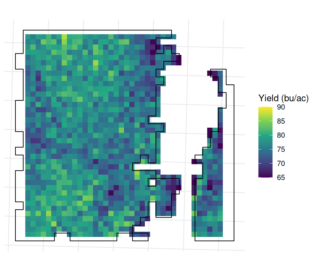

Figure 3.3: The wheat field gridded to 20 m, with the field boundary.

library(sf)
library(terra)

pts_f1 <- clean_f1 |>
  st_as_sf(coords = c("longitude", "latitude"), crs = 4326) |>
  st_transform(32613) |>
  vect()
yr_f1 <- rasterize(pts_f1, rast(pts_f1, resolution = 20),
                   field = "yield", fun = mean)

clean_f1 |>
  summarise(
    n          = n(),
    mean_yield = mean(yield),
    sd_yield   = sd(yield),
    mean_moist = mean(moisture)
  )

## Harvested acres from the cells, against the boundary
cells_f1 <- sum(!is.na(values(yr_f1)))
cells_f1 * 400 / 4046.86

bnd_f1 <- st_read("data/example_wheat_boundary.geojson", quiet = TRUE) |>
  st_transform(32613)
as.numeric(st_area(bnd_f1)) / 4046.86

> library(sf)
> library(terra)
> 
> pts_f1 <- clean_f1 |>
+   st_as_sf(coords = c("longitude", "latitude"), crs = 4326) |>
+   st_transform(32613) |>
+   vect()
> yr_f1 <- rasterize(pts_f1, rast(pts_f1, resolution = 20),
+                    field = "yield", fun = mean)
> 
> clean_f1 |>
+   summarise(
+     n          = n(),
+     mean_yield = mean(yield),
+     sd_yield   = sd(yield),
+     mean_moist = mean(moisture)
+   )
# A tibble: 1 × 4
      n mean_yield sd_yield mean_moist
  <int>      <dbl>    <dbl>      <dbl>
1 23288       76.2     11.9       10.8
> 
> ## Harvested acres from the cells, against the boundary
> cells_f1 <- sum(!is.na(values(yr_f1)))
> cells_f1 * 400 / 4046.86
[1] 114.0637
> 
> bnd_f1 <- st_read("data/example_wheat_boundary.geojson", quiet = TRUE) |>
+   st_transform(32613)
> as.numeric(st_area(bnd_f1)) / 4046.86
[1] 123.1617

After cleaning, the wheat field has 23,288 usable readings with an average yield of 76.2 bu/ac and average moisture of 10.9%. These readings fall in 1,154 grid cells.

Here the area covered by the grid differs more from the boundary area. The grid covers 114.1 acres, compared with 123.2 acres inside the boundary. Looking at the map helps explain the difference. This field is two separate blocks of wheat in the same quarter: a large block and a narrow strip to the east. Much of the roughly 9-acre difference occurs around their edges.

A grid only approximates the shape of the harvested area. Some cells along the edge have no recorded point and are left empty, even if the header cut part of that cell. Other cells contain a reading and are drawn as a whole square, extending a little beyond the boundary. Both are consequences of representing an irregular field with 20 m squares, and they are particularly noticeable around the narrow strip.

We can report an average of 76.2 bu/ac for the retained readings and an estimated area of about 114 acres from the grid. If we want to estimate total production, we also need to decide which area to use. State that choice alongside the result, since the grid area and the boundary area give different totals.

Section 4 — Merging with satellite data

In this section, we will combine the harvest data with satellite data and fit a simple model. You should be able to:

1. Merge NDVI and yield data by putting them on the same grid.
2. Calculate the correlation between NDVI and yield for each week and explain why the relationship differs through the season.
3. Fit a linear model using NDVI from one or more weeks to predict yield, and interpret the results.

The two examples use different formats for the satellite data. For the barley field, we have a table with a row for each pixel and date. For the wheat field, we have a raster for each week. In both cases, we need to make sure that each yield value is matched with NDVI from the same area of ground.

Example 1 — the barley field, NDVI as a long table

The file example_barley_ndvi.csv contains the columns easting, northing, date and ndvi. Each row gives the NDVI for one pixel on one date. We will use those coordinates to put the NDVI observations on the same grid as the yield readings.

Step 1: create the yield grid, then use it as the template for NDVI.

library(tidyverse)
library(sf)
library(terra)

barley <- read_csv("data/example_barley.csv") |>
  filter(!is.na(yield_bu_ac), yield_bu_ac > 0, yield_bu_ac < 300, swath_ft >= 39)

pts  <- barley |>
  st_as_sf(coords = c("longitude", "latitude"), crs = 4326) |>
  st_transform(32613) |>
  vect()
grid <- rast(pts, resolution = 20)
yield_r <- rasterize(pts, grid, field = "yield_bu_ac", fun = mean)

## The NDVI arrives long: one row per pixel per date
ndvi <- read_csv("data/example_barley_ndvi.csv")
n_distinct(ndvi$date)

## Some dates are mostly cloud. Count the pixels before trusting a date
ndvi |> count(date) |> arrange(n) |> head(8)

> library(tidyverse)
> library(sf)
> library(terra)
> 
> barley <- read_csv("data/example_barley.csv") |>
+   filter(!is.na(yield_bu_ac), yield_bu_ac > 0, yield_bu_ac < 300, swath_ft >= 39)
Rows: 37957 Columns: 12
── Column specification ────────────────────────────────────────────────────────
Delimiter: ","
chr (3): field, crop, variety
dbl (9): seconds_in, yield_bu_ac, moisture_pct, speed_mph, heading_deg, elev...

ℹ Use `spec()` to retrieve the full column specification for this data.
ℹ Specify the column types or set `show_col_types = FALSE` to quiet this message.
> 
> pts  <- barley |>
+   st_as_sf(coords = c("longitude", "latitude"), crs = 4326) |>
+   st_transform(32613) |>
+   vect()
> grid <- rast(pts, resolution = 20)
> yield_r <- rasterize(pts, grid, field = "yield_bu_ac", fun = mean)
> 
> ## The NDVI arrives long: one row per pixel per date
> ndvi <- read_csv("data/example_barley_ndvi.csv")
Rows: 22818 Columns: 5
── Column specification ────────────────────────────────────────────────────────
Delimiter: ","
chr  (1): field
dbl  (3): easting, northing, ndvi
date (1): date

ℹ Use `spec()` to retrieve the full column specification for this data.
ℹ Specify the column types or set `show_col_types = FALSE` to quiet this message.
> n_distinct(ndvi$date)
[1] 21
> 
> ## Some dates are mostly cloud. Count the pixels before trusting a date
> ndvi |> count(date) |> arrange(n) |> head(8)
# A tibble: 8 × 2
  date           n
  <date>     <int>
1 2026-07-23   129
2 2026-08-02   233
3 2026-09-21   278
4 2026-08-29   295
5 2026-08-19   322
6 2026-09-13   447
7 2026-08-07   658
8 2026-09-26  1131

Seven of the 21 dates have fewer than 1,000 pixels because much of the image was masked by cloud. A correlation using one of those dates would describe only the part of the field that was visible. For this example, we will keep dates with more than 1,000 pixels and group the observations by week.

## Keep the dates that actually cover the field, and label them by week
good <- ndvi |> count(date) |> filter(n > 1000) |> pull(date)
ndvi_ok <- ndvi |>
  filter(date %in% good) |>
  mutate(wk = paste0("W", isoweek(as.Date(date))))

weeks <- sort(unique(ndvi_ok$wk))
weeks

## Rasterize each week onto the SAME template as the yield.  Passing grid as
## the template is what guarantees the cells line up -- two rasters at the same
## resolution need not share an origin
layers <- lapply(weeks, function(w) {
  sub <- filter(ndvi_ok, wk == w)
  v <- vect(as.matrix(sub[, c("easting", "northing")]),
            type = "points", crs = "EPSG:32613")
  values(v) <- data.frame(ndvi = sub$ndvi)
  rasterize(v, grid, field = "ndvi", fun = mean)
})

stack <- rast(c(list(yield_r), layers))
names(stack) <- c("yield", weeks)

cells <- as.data.frame(stack, na.rm = FALSE) |> filter(!is.na(yield))
nrow(cells)

> ## Keep the dates that actually cover the field, and label them by week
> good <- ndvi |> count(date) |> filter(n > 1000) |> pull(date)
> ndvi_ok <- ndvi |>
+   filter(date %in% good) |>
+   mutate(wk = paste0("W", isoweek(as.Date(date))))
> 
> weeks <- sort(unique(ndvi_ok$wk))
> weeks
 [1] "W18" "W19" "W21" "W22" "W28" "W29" "W30" "W31" "W38" "W39" "W40"
> 
> ## Rasterize each week onto the SAME template as the yield.  Passing grid as
> ## the template is what guarantees the cells line up -- two rasters at the same
> ## resolution need not share an origin
> layers <- lapply(weeks, function(w) {
+   sub <- filter(ndvi_ok, wk == w)
+   v <- vect(as.matrix(sub[, c("easting", "northing")]),
+             type = "points", crs = "EPSG:32613")
+   values(v) <- data.frame(ndvi = sub$ndvi)
+   rasterize(v, grid, field = "ndvi", fun = mean)
+ })
> 
> stack <- rast(c(list(yield_r), layers))
> names(stack) <- c("yield", weeks)
> 
> cells <- as.data.frame(stack, na.rm = FALSE) |> filter(!is.na(yield))
> nrow(cells)
[1] 1525

Step 2: calculate the correlation between yield and each week’s NDVI.

## use = "complete.obs" because a cloudy corner leaves NAs in some weeks
week_cor <- sapply(weeks, function(w) cor(cells$yield, cells[[w]],
                                          use = "complete.obs"))
round(sort(week_cor, decreasing = TRUE), 3)

> ## use = "complete.obs" because a cloudy corner leaves NAs in some weeks
> week_cor <- sapply(weeks, function(w) cor(cells$yield, cells[[w]],
+                                           use = "complete.obs"))
> round(sort(week_cor, decreasing = TRUE), 3)
   W29    W28    W31    W30    W40    W21    W39    W22    W38    W19    W18 
 0.618  0.558  0.534  0.505 -0.043 -0.106 -0.211 -0.330 -0.385 -0.432 -0.456 

The strongest positive correlation is in W29, at r = 0.618. Weeks 28 to 31, in mid to late July, all have correlations between 0.50 and 0.62. Outside that period, the correlations are weak or negative. In May, W18 and W19 are around −0.45. At that point there is little crop cover, so NDVI is largely responding to the soil rather than the crop canopy. The areas with higher early NDVI later yield less. As in the chapter, we need to consider the stage of the crop when interpreting the index.

Step 3: fit yield as a function of week 29 NDVI.

m <- lm(yield ~ W29, data = cells)
summary(m)

> m <- lm(yield ~ W29, data = cells)
> summary(m)

Call:
lm(formula = yield ~ W29, data = cells)

Residuals:
    Min      1Q  Median      3Q     Max 
-38.454  -5.983  -1.106   4.909  49.532 

Coefficients:
            Estimate Std. Error t value Pr(>|t|)    
(Intercept)  -27.416      4.661  -5.882 5.19e-09 ***
W29          141.931      5.092  27.871  < 2e-16 ***
---
Signif. codes:  0 '***' 0.001 '**' 0.01 '*' 0.05 '.' 0.1 ' ' 1

Residual standard error: 10.58 on 1260 degrees of freedom
  (263 observations deleted due to missingness)
Multiple R-squared:  0.3814,	Adjusted R-squared:  0.3809 
F-statistic: 776.8 on 1 and 1260 DF,  p-value: < 2.2e-16

The NDVI coefficient is 141.9. A difference of 0.1 in W29 NDVI is therefore associated with about 14 bu/ac higher yield. The intercept, −27.4, is the predicted yield at NDVI zero. Since the observations in this field are nowhere near zero, we should not give that intercept an agronomic interpretation.

The R² is 0.38, so the model explains a little over a third of the variation in yield between cells. There is useful information in the July image, but much of the variation remains unexplained. Other growing conditions and measurement noise can contribute to that remaining variation; the model does not tell us how much comes from each.

Example 2 — the wheat field, NDVI as weekly rasters

For the wheat field, we have one GeoTIFF raster per week. We can use project() to put these rasters on the yield grid. We will then compare a model using one week of NDVI with a model using three weeks, to see how much the additional images improve the fit.

library(tidyverse)
library(sf)
library(terra)

wheat <- read_csv("data/example_wheat.csv") |>
  filter(yield > 0, yield < 300, width_ft >= 39)

pts  <- wheat |>
  st_as_sf(coords = c("longitude", "latitude"), crs = 4326) |>
  st_transform(32613) |>
  vect()
grid <- rast(pts, resolution = 20)
yield_r <- rasterize(pts, grid, field = "yield", fun = mean)

## Read the three weeks and put them on the yield grid.  project() with a
## raster as the target resamples onto that exact grid
wk_file <- function(w) sprintf("data/example_wheat_ndvi/wheat_ndvi_2026-%s.tif", w)
nd <- rast(sapply(c("W29", "W30", "W31"), wk_file)) |> project(yield_r)
names(nd) <- c("W29", "W30", "W31")

cells <- as.data.frame(c(yield_r, nd), na.rm = FALSE) |>
  rename(yield = mean) |>
  filter(!is.na(yield))
nrow(cells)

> library(tidyverse)
> library(sf)
> library(terra)
> 
> wheat <- read_csv("data/example_wheat.csv") |>
+   filter(yield > 0, yield < 300, width_ft >= 39)
Rows: 24637 Columns: 12
── Column specification ────────────────────────────────────────────────────────
Delimiter: ","
chr  (3): field, crop, variety
dbl  (8): longitude, latitude, yield, moisture, speed_mph, width_ft, elevati...
dttm (1): iso_time

ℹ Use `spec()` to retrieve the full column specification for this data.
ℹ Specify the column types or set `show_col_types = FALSE` to quiet this message.
> 
> pts  <- wheat |>
+   st_as_sf(coords = c("longitude", "latitude"), crs = 4326) |>
+   st_transform(32613) |>
+   vect()
> grid <- rast(pts, resolution = 20)
> yield_r <- rasterize(pts, grid, field = "yield", fun = mean)
> 
> ## Read the three weeks and put them on the yield grid.  project() with a
> ## raster as the target resamples onto that exact grid
> wk_file <- function(w) sprintf("data/example_wheat_ndvi/wheat_ndvi_2026-%s.tif", w)
> nd <- rast(sapply(c("W29", "W30", "W31"), wk_file)) |> project(yield_r)
> names(nd) <- c("W29", "W30", "W31")
> 
> cells <- as.data.frame(c(yield_r, nd), na.rm = FALSE) |>
+   rename(yield = mean) |>
+   filter(!is.na(yield))
> nrow(cells)
[1] 1154

## One week on its own
m1 <- lm(yield ~ W30, data = cells)
summary(m1)$r.squared
coef(m1)

## All three together
m3 <- lm(yield ~ W29 + W30 + W31, data = cells)
summary(m3)

> ## One week on its own
> m1 <- lm(yield ~ W30, data = cells)
> summary(m1)$r.squared
[1] 0.227754
> coef(m1)
(Intercept)         W30 
   36.87942    55.00359 
> 
> ## All three together
> m3 <- lm(yield ~ W29 + W30 + W31, data = cells)
> summary(m3)

Call:
lm(formula = yield ~ W29 + W30 + W31, data = cells)

Residuals:
     Min       1Q   Median       3Q      Max 
-13.0689  -2.1132   0.0073   2.0728  15.7397 

Coefficients:
            Estimate Std. Error t value Pr(>|t|)    
(Intercept)   39.145      2.238  17.492  < 2e-16 ***
W29          -23.031      1.990 -11.576  < 2e-16 ***
W30           67.678      3.045  22.224  < 2e-16 ***
W31            6.006      1.292   4.649 3.73e-06 ***
---
Signif. codes:  0 '***' 0.001 '**' 0.01 '*' 0.05 '.' 0.1 ' ' 1

Residual standard error: 3.268 on 1150 degrees of freedom
Multiple R-squared:  0.3249,	Adjusted R-squared:  0.3231 
F-statistic: 184.5 on 3 and 1150 DF,  p-value: < 2.2e-16

Using W30 alone gives an R² of 0.228, while using all three weeks gives 0.325. The three-week model fits these observations better. However, when we fit the same observations, adding predictors cannot lower R². We would need to check prediction errors on data left out of fitting before concluding that the additional weeks improve prediction.

Notice that the W29 coefficient is −23.0 and statistically significant. The negative sign may seem surprising if we expect greener areas to yield more. Let’s look at W29 on its own and at how the three weeks relate to each other.

## On its own, what does W29 say?
cor(cells$yield, cells$W29, use = "complete.obs")

## The three weeks are images of the same crop a week apart
round(cor(cells[, c("W29", "W30", "W31")], use = "complete.obs"), 3)

> ## On its own, what does W29 say?
> cor(cells$yield, cells$W29, use = "complete.obs")
[1] -0.08265511
> 
> ## The three weeks are images of the same crop a week apart
> round(cor(cells[, c("W29", "W30", "W31")], use = "complete.obs"), 3)
       W29   W30    W31
W29  1.000 0.388 -0.046
W30  0.388 1.000  0.075
W31 -0.046 0.075  1.000

On its own, W29 has a weak negative correlation with yield, −0.083. W29 and W30 are also related to each other, with a correlation of 0.388. Remember that in the three-week model, each coefficient describes the relationship with one week’s NDVI holding the other weeks fixed. The W29 coefficient therefore compares cells with different W29 greenness but the same W30 and W31 values. That is a different comparison from asking whether greener cells generally yield more, and it is harder to give a simple agronomic interpretation.

For explaining the relationship between NDVI and yield, I would report the one-week model because it is easier to interpret. If the aim is prediction, I would compare the two models on observations left out of fitting. The roughly 0.10 increase in R² tells us that three weeks fit the available data better, but it does not tell us how much they improve predictions on new data.