2 Working with Data in Excel
The first chapter covered how a spreadsheet works. This chapter moves from simple calculations to working with real data in Excel: calculating statistics for subsets of observations, pulling information from one table into another, sorting and filtering data, and summarizing large datasets by category.
2.1 Conditional Functions
So far, our formulas have performed calculations without making decisions: multiply these two values, add this range, calculate its average. Conditional functions let a formula make a decision, or apply a calculation only when some condition is met.
IF
IF is the function that makes a decision. It looks at a condition and returns one of two values depending on whether that condition is true. The IF function has three arguments that are separated by commas: (1) the condition to test, (2) the value to return if the condition is true, and (3) the value to return if the condition is false. Both the condition and the values returned can reference other cells.
In the following example, IF tests whether the value in D2 is greater than 50. If the condition is true, it returns the text Yes; if the condition is false, it returns the text No.
=IF(D2>50, "Yes", "No")Column E of the workbook below uses exactly this formula to label each field "Yes" or "No". Note the quotation marks: text inside a formula always needs them. The returned values can also reference cells – =IF(D2>50, C2, "No") would return the field’s acres when the condition is true.
Download this workbook
Open online (File → Save a Copy to view formulas and edit). The workbook includes a practice sheet to fill in yourself.
Sometimes one test is not enough. Because the true and false arguments can hold anything, they can hold another IF. To flag only the fields that are both over 50 bu/ac and canola:
=IF(D2>50, IF(B2="Canola", "Yes", "No"), "No")Read it from the outside in. If the yield clears 50, Excel moves to the inner IF and checks the crop; if it does not, the whole thing returns No without looking further. Nesting more than two or three deep gets hard to read, and at that point a helper column is usually clearer.
COUNTIF, SUMIF, and AVERAGEIF
COUNT, SUM, and AVERAGE calculate across an entire range. Each has a conditional version that performs the calculation using only observations that meet a specified condition – the average yield on canola fields, for example, or the number of fields yielding more than 60 bushels per acre.
COUNTIF takes two arguments: the range to test and the condition to test for. SUMIF and AVERAGEIF take a third argument: the range containing the values to sum or average. Here are three examples:
=COUNTIF(B2:B9, "Canola")
=SUMIF(B2:B9, "Canola", C2:C9)
=AVERAGEIF(B2:B9, "Canola", D2:D9)
The first formula counts the fields where column B contains Canola. The second identifies those same fields and adds up their acres from column C. For example, if B2 and B4 both contain Canola, the SUMIF formula will include C2+C4. AVERAGEIF works in the same way, except that it averages the corresponding values rather than adding them.
The two ranges must be the same size, but they do not technically need to contain the same row numbers. Excel matches the cells by their position within each range. For example, you could write: =SUMIF(B2:B9, "Canola", D12:D19). Here, B2 is paired with D12, B3 with D13, B4 with D14, and so on. If B2 and B4 contain Canola, Excel would therefore add D12+D14.
In practice, the ranges will usually cover the same rows of a dataset. The important point is that Excel matches their relative positions, not their row numbers.
Examples of these functions are in rows 12-16 of the workbook above.
COUNTIFS, SUMIFS, and AVERAGEIFS
COUNTIF and its relatives test one condition. Often you need two. In a dataset with one row per province, crop and year, “the average canola yield in Ontario” is a question about two columns at once, and no single-condition function can answer it.
In the following formula
=COUNTIFS(A2:A1068, 2023, C2:C1068, "Canola")Excel will include row 2 in its count if A2 contains 2023 and C2 contains Canola, row 3 if A3 contains 2023 and C3 contains Canola, and so on. It will not include row 2 if either condition fails. The formula will return the number of rows that meet both conditions.
The argument order for AVERAGEIFS and SUMIFS are a bit different from AVERAGEIF and SUMIF. The range being averaged comes first, followed by pairs: a range to test, then the condition to test it for. Add as many pairs as you need and Excel keeps only the rows that satisfy all of them.
For eaxmple in,
=AVERAGEIFS(E2:E1068, C2:C1068, "Canola", B2:B1068, "Ontario")Excel will include E2 in the acverage if C2 contains Canola and B2 contains Ontario; it will include E3 if C3 contains Canola and B3 contains Ontario, and so on. The formula returns the average of all the values in column E that meet both conditions.
All the conditional functions can use comparisons as well as exact matches. To average canola yields only in years after 2020:
=AVERAGEIFS(E2:E1068, C2:C1068, "Canola", A2:A1068, ">2020")- Excel for Dummies – Microsoft 365 Excel for Dummies, the chapters on logical functions (
IF) and on conditional counting/summing. - Microsoft Support – IF function, COUNTIF, SUMIF, AVERAGEIF.
- Video (IF function) – IF function in Excel tutorial.
- Video (COUNTIF / SUMIF / AVERAGEIF) – How to use SUMIF, COUNTIF, and AVERAGEIF in Excel.
- Video (broader formulas course) – Kevin Stratvert, Excel formulas and functions – full course (includes an IF-function section).
2.2 Lookup Functions
Data often arrive split across tables. You might have yields by field in one table and crop prices in another but need both pieces of information for your analysis. A lookup lets us use information in one table to bring a corresponding value into another.
XLOOKUP lets us look up a value. It takes three main arguments: the value to find, the range to search and the range containing the value to return. For example:
=XLOOKUP(B11, $A$5:$A$7, $B$5:$B$7)Excel searches $A$5:$A$7 for the crop named in B11, finds its position and returns the value from the same position in $B$5:$B$7. Note the $ signs: the crop being looked up changes from row to row, but the price table stays in place, so its ranges are locked.
If there are multiple matches – for example, if Canola appears twice in the price list – XLOOKUP returns the value associated with the first match. The value you look up should therefore identify a unique observation in the lookup table.
The workbook below has two tables: a short crop-price list at the top and the field data underneath. Column E uses XLOOKUP to find the price for each field’s crop and bring it across, with the formula shown in column F.
Download this workbook
Open online (File → Save a Copy to view formulas and edit). The workbook includes a practice sheet to fill in yourself.
Looking up values using multiple keys
Sometimes one column is not enough to identify an observation. Suppose we have crop yields and crop prices for several years. Crop alone is not a unique key because Canola appears once in every year. To find the appropriate price, we have to match both crop and year.
The clearest way to do this in Excel is to create a helper column in each dataset that combines the two keys. If crop is in B2 and year is in A2, enter:
=B2 & "|" & A2This creates values such as Canola|2023 and Wheat|2024. The separator matters: without it, different pairs of values can sometimes produce the same combined key. Create the same helper column, using the same order and separator, in the price table. You can then use a regular XLOOKUP to match the combined key in the yield table to the combined key in the price table:
=XLOOKUP(F2, $H$2:$H$7, $I$2:$I$7)Here, F2 contains the combined crop-year key for a yield observation, column H contains the matching keys in the price table and column I contains the prices to return. Before using the lookup, confirm that each combined key appears only once in the price table. If a key is duplicated, XLOOKUP silently returns the first match.
It is possible to combine the keys directly inside XLOOKUP, but explicit helper columns are easier to inspect. You can see whether both tables created the same keys and identify spelling, spacing or type problems before relying on the result.
An unmatched XLOOKUP returns #N/A. If every row returns #N/A, check that the helper columns use the same order and separator, that text does not contain stray spaces and that the corresponding values have the same type.
- Excel for Dummies – Microsoft 365 Excel for Dummies, the chapter on lookup and reference functions.
- Microsoft Support – VLOOKUP, XLOOKUP, INDEX, MATCH.
- Video (XLOOKUP) – Leila Gharani, How an Excel pro uses XLOOKUP (XLOOKUP vs VLOOKUP and INDEX/MATCH).
- Video (VLOOKUP for beginners) – Kevin Stratvert, VLOOKUP in Excel – step-by-step tutorial.
- Video (INDEX/MATCH) – Leila Gharani, The definitive guide to INDEX and MATCH.
2.3 Sorting and Filtering
Sorting and filtering are different from the functions we have used so far. Rather than calculating a new value, they change how the data in a worksheet is displayed and organized. The examples below use the same eight fields as before.
Sorting
Sorting changes the order of the rows in a dataset. Click any cell in the column you want to sort by, then use Sort & Filter on the Home tab.
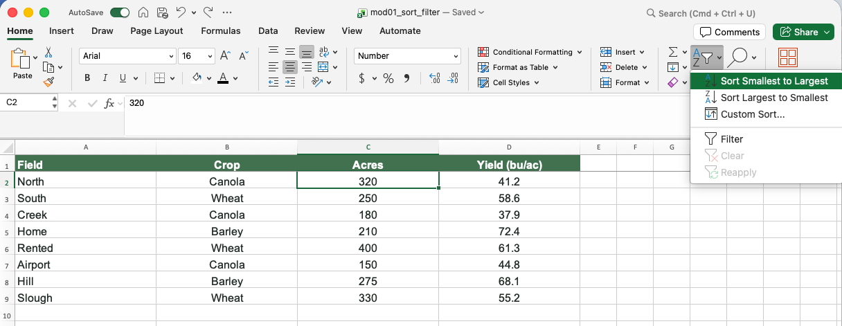
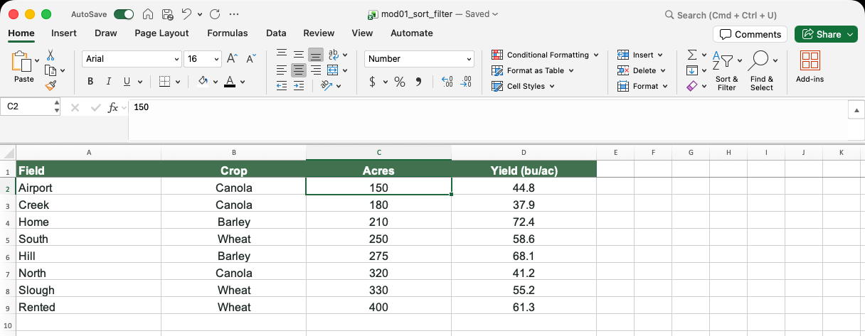
Sorting by Acres, smallest to largest, gives this:
Filtering
Filtering temporarily hides observations that do not meet a condition. Turn filtering on from the same menu:
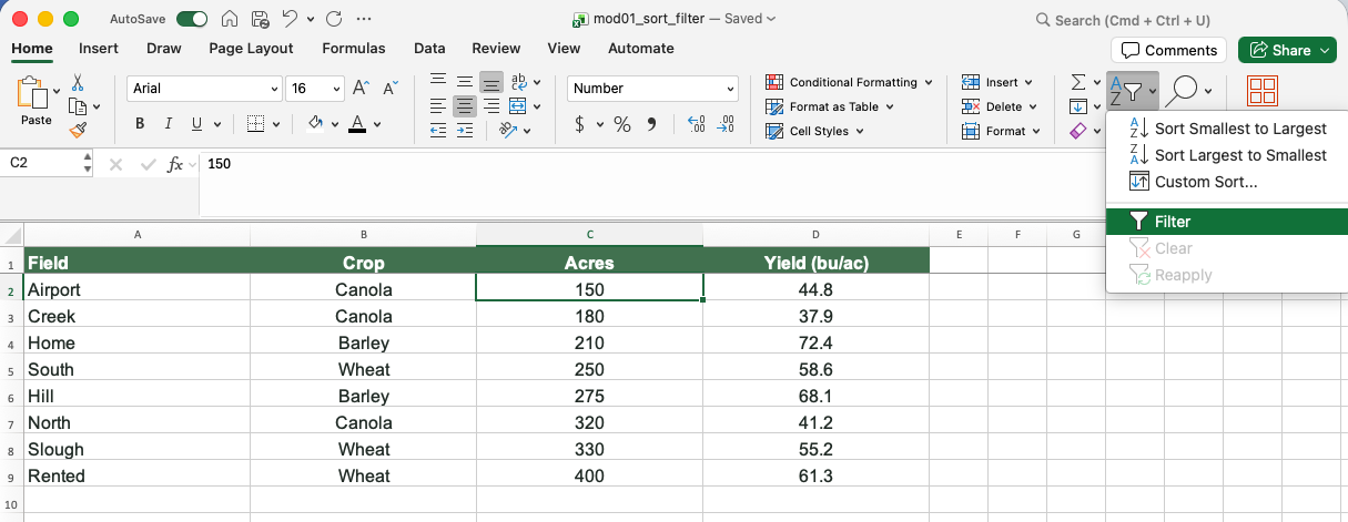
Clicking one of those arrows opens a panel containing the values in that column:
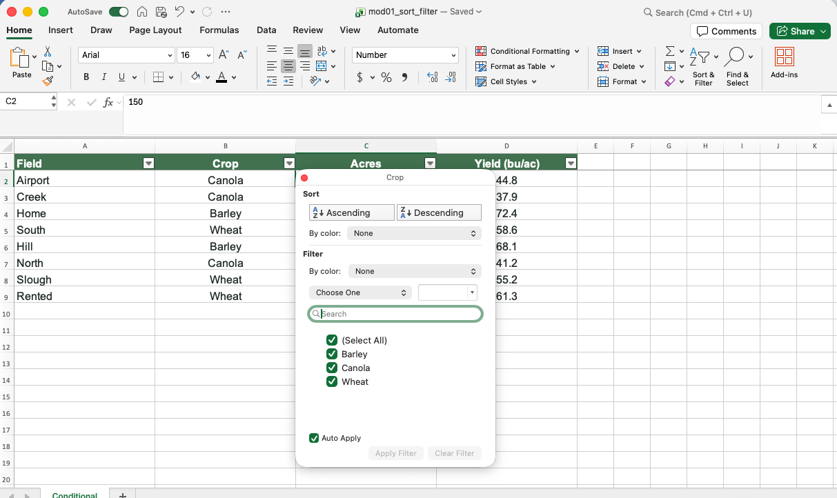
If we select only Canola, Excel hides the other observations:
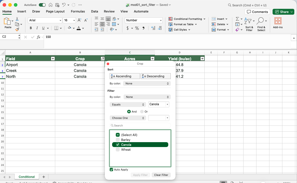
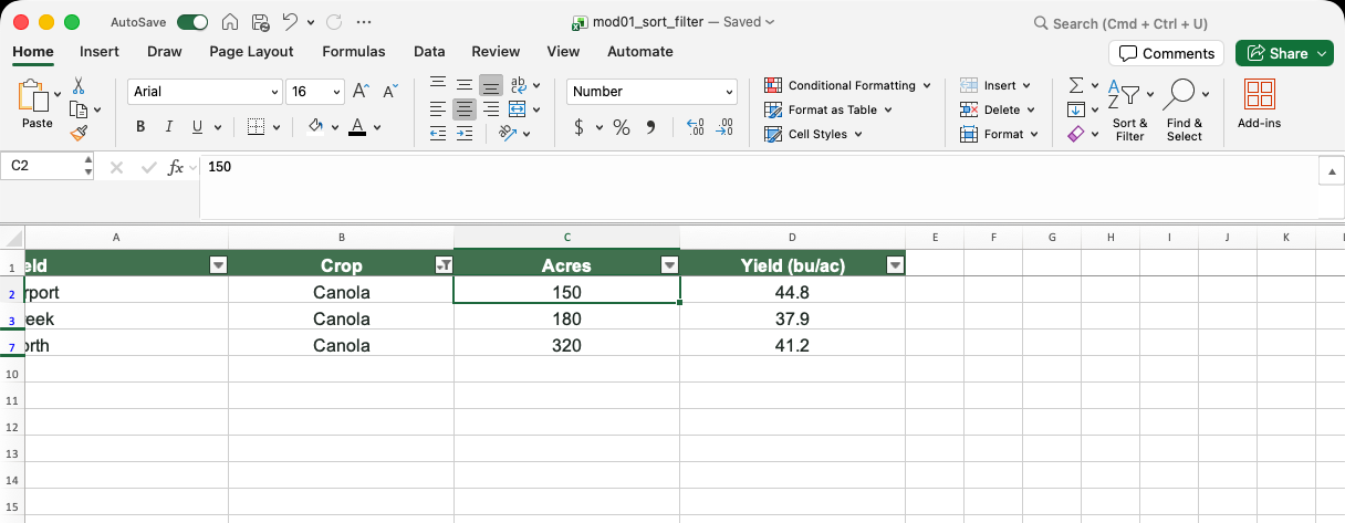
Notice that the row numbers are no longer consecutive. The gaps indicate that some rows are hidden by the filter. This is an easy way to tell that you are viewing only part of the dataset. Nothing has been deleted – clearing the filter makes all of the observations visible again.
Ctrl+Shift+L on Windows or ⌘⇧F on a Mac toggles filters on and off.
Download the sorting and filtering workbook to sort and filter the fields yourself. The workbook includes a practice sheet to fill in.
Note that filters hide rows from you, but those hidden rows are still part of the datasets and would be included in formulas. If you filter a column to show only 2023 and then write =AVERAGE(E2:E10650), Excel still averages every row – including the hidden ones. To calculate a statistic for a subset of the data, you can use the conditional functions we covered earlier. Or, if you want to only use the filtered data for some analysis you can copy and paste that data into a new worksheet. :::
- Excel for Dummies – Microsoft 365 Excel for Dummies, the chapter on sorting and filtering data.
- Microsoft Support – Sort data in a range or table and Filter data in a range or table.
- Video (right-click method) – Excel sort and filter: skip the ribbon, use right-click.
- Video (basics) – The Organic Chemistry Tutor, Excel sorting and filtering data.
2.4 Wide vs. Long Data
The same data can be arranged in different ways, and the shape of the data affects how easily we can work with it. Two common shapes are wide and long. The workbook below contains the same data in both forms on separate worksheets, with an explanation of the difference on the first worksheet.
Download this workbook · Open online (File → Save a Copy to view formulas and edit)
In the wide table, crop names appear as column headings – three crops, three columns of yields. In the long table, Crop is itself a column, with the crop names appearing as values, while all of the yields are stacked in a single Yield column. The information is the same; only its shape has changed.
Wide data is often easy for people to read and convenient for calculations involving individual columns. If you want the average canola yield, for example, you can simply average the Canola column. Long data is particularly useful when you want to group or summarize observations by a variable. In the long table, Crop is a variable that Excel can use to divide the observations into groups.
This becomes important for PivotTables. If we want a PivotTable showing average yield by crop, Excel needs Crop to be a field that it can group by. The long format provides exactly that: one column identifying the crop and another containing the yield.
- R for Data Science (Wickham) – the Data tidying chapter is the definitive treatment of tidy data and the wide/long distinction (we return to this in Module 3).
- Video (concept + reshaping) – Riffomonas Project, Reshaping data to be long or wide with pivot_longer and pivot_wider. Uses R, but the idea of wide vs. long is exactly what we need here.
2.5 PivotTables
PivotTables are best understood by seeing them in action. The video above shows one being built – I would suggest wathicn the video before reading on.
A PivotTable summarizes a dataset by category – average yield by crop, total acres by year, or average yield by crop and year – without requiring you to write formulas. This is one reason why long data is so useful: the variables stored in columns can become the categories that a PivotTable groups by.
You build a PivotTable by dragging the variable you want to group by into one box and the variable you want to summarize into another. The name comes from how easily you can pivot the resulting table: put crops down the rows and years across the columns, swap them, or add another variable to create more detailed groups – all by dragging fields to different positions.
The workbook below puts this to work. Its Data tab contains the full variety-yield file: one row per risk zone, crop, variety and year – 14,700 rows, far too many to usefully inspect one at a time. The PivotTable tab summarizes them in one table: average barley yield by variety and year, with the risk zone available as a filter. Swap Crop in the filter, or drag Risk_Zone into Rows, and the same 14,700 rows answer a different question.
Download this workbook
Open online (File → Save a Copy to view formulas and edit)
To build one yourself, click any cell inside the data and select Insert → PivotTable. Put the PivotTable on a new worksheet. Excel gives you an empty table and a list of the variables in your data. Drag a variable into Rows to define the groups, and drag the variable you want to summarize into Values. Drag another categorical variable into Columns to create a two-way table. The Filters box lets you restrict the entire summary to particular observations.
Be careful about how Excel summarizes the variable in Values. Excel will often default to adding the values together. If you put Yield there, for example, Excel may report the sum of all the yields – a number with no useful interpretation. Instead, click the value and use Summarize Values By to choose the statistic you actually want, such as Average. The PivotTable tab in the workbook is built this way, so you can compare your results with it.
Two other features are useful. Show Values As can display values as percentages of a row, column, or grand total. And double-clicking a value inside a PivotTable creates a new worksheet containing the observations behind that number. This is a quick way to investigate a result that looks surprising.
You can drag the same field into Values twice and summarize it two different ways. Yield as Average and Yield as Count puts the mean beside the number of observations behind it, which tells you how much data each average rests on.
The dropdown on a row field holds more than the list of values. Value Filters keep only the rows whose summarized number meets a condition – varieties with at least 30 reports, say – which is easier than unchecking several hundred boxes by hand. Label Filters do the same on the names themselves.
Selecting a cell in a PivotTable and choosing Insert → PivotChart creates a chart tied to the table. Filter or rearrange the PivotTable and the chart follows, which is the advantage over copying numbers into an ordinary chart. Give it a title and label the axes as you would any chart.
Finally, before interpreting any summary, check the units. The crops in this workbook are not all measured in the same units: cereals and canola are in bushels per acre, while pulse crops such as lentils and chickpeas are reported in pounds per acre. A PivotTable that averages yield across all crops mixes the two. Excel will happily average pounds per acre together with bushels per acre and return a number – but that number has no meaningful interpretation. Keep Crop in the filter, or in Rows, so every cell of the summary is one crop in one unit.
- Excel for Dummies – Microsoft Excel Data Analysis for Dummies (3rd ed.), the PivotTable chapters (this is one of the book’s strongest topics).
- Microsoft Support – Create a PivotTable to analyze worksheet data.
- Video (beginner walkthrough) – Kevin Stratvert, How to create a pivot table in Excel.
2.6 Working Efficiently in Excel
Once datasets get large, you will start finding it clunky to navigate the worksheet with a mouse. Learning to navigate with keyboard shortcuts will make life much easier.
The most useful shortcut is Command (⌘) + arrow on a Mac or Ctrl + arrow on Windows. It jumps to the edge of the current block of data. If you are at the top of a column containing 10,000 observations, for example, ⌘+↓ or Ctrl+↓ takes you to the bottom almost instantly.
Adding Shift selects everything along the way. This is particularly useful when selecting a range for a formula: instead of dragging down thousands of rows, click the first value and use ⌘+Shift+↓ on a Mac or Ctrl+Shift+↓ on Windows.
If there is a blank cell partway down a column, Excel may stop there. This can actually be useful – an unexpected stop may alert you to a blank in your data.
A Few More Time-Savers
Use the fill handle. The small square at the bottom-right corner of a selected cell lets you copy a formula to adjacent cells. Drag it down, or double-click it to fill the formula down alongside a neighbouring column of data. Relative and absolute references behave as described in Relative and Absolute References.
Freeze your headings. For a long dataset, use View → Freeze Panes → Freeze Top Row to keep the variable names visible as you scroll.
Use Undo.
⌘+Zon a Mac orCtrl+Zon Windows reverses your last action. This is particularly useful when experimenting with sorting, formulas, or formatting.Use AutoSum. The Σ AutoSum button on the Home tab will usually identify a nearby range of numbers and write the
SUMformula for you. Always check that Excel selected the range you intended.Paste values when you need the result rather than the formula. Copy the cells and use Paste Special → Values. The pasted cells contain the resulting values rather than the formulas that produced them.