9 Merging Data

The data you need to answer one question often arrive in several tables. For example, suppose we wanted to understand the relationship between RM yields and precipitation. The yield data would come in one table, and the precipitation data would likely come in another. To answer our question, we would need to merge or join these tables.

The data used in this chapter are:

rm_yields_2015_2024.csv – one row per RM per year. It contains 2,950 rows for ten years and six crops. Yields are measured in bushels per acre.
station_precip.csv – one row per weather station per year. It contains May to August precipitation for sixteen stations and a count of days with no reading.
rm_lookup.csv – one row per RM. It contains the RM name, census division, 2021 population and the closest of the sixteen weather stations.

We will do two merges:

Merge the RM yields with the RM lookup. This will give us a dataset containing the closest weather station for each yield observation.
Merge the dataset from step 1 with the weather station data. This will give us the growing-season precipitation for each observation.

Keys

A key is a column, or set of columns, used to identify and match rows across datasets. When we merge, we say that we merge on the key. The key must be present in both datasets.

In the three tables above, the keys for the two merges are:

RM yields to RM lookup: RM.
The resulting dataset to weather-station data: weather station and year.

One-to-one, many-to-one and many-to-many

There are three types of merges:

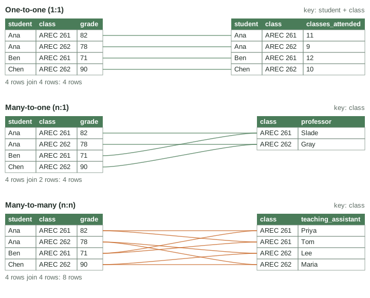
Figure 9.1: Three kinds of merge. Each line connects a grades row to the row it matches.

One-to-one (1:1). Each key value appears once in both tables. Grades and attendance both have one row per student-class, so the merged table has the same number of rows as either input.
Many-to-one (n:1). Values in the key column may repeat in one dataset but are unique in the other. In this example, students take many classes, so each student appears multiple times in the table on the left. Each class has a single professor, however, so each class appears only once in the table on the right.
Many-to-many (n:n). Values in the key column repeat in both datasets. In the figure, students take multiple classes (the table on the left), and each class can have multiple teaching assistants (the table on the right).

Before joining, decide which relationship you expect. Then compare the row counts before and after.

Both of our merges will be many-to-one:

The RM yields dataset contains many observations for the same RM, but the RM lookup contains only one row for each RM.
The merged dataset from step 1 contains many observations with the same closest weather station and year, but the weather-station dataset contains only one observation for each station and year.

9.1 Merging in Excel

Video walkthrough of this section

In Chapter 2, we used XLOOKUP to bring values from one table into another (Section 2.2). That approach is useful for a quick lookup. Here, we will use Power Query because it records the merge as a repeatable series of steps and can match on several columns directly.

Begin by importing rm_yields_2015_2024.csv and rm_lookup.csv with Data > Get Data > From Text/CSV > Transform Data. In the Power Query editor:

Load the RM yield data using Power Query, transforming the data to longer format as we did before.
Choose Power Query, select import csv, and select the RM lookup table.
Select transform data. You will now see two queries on your left hand side (Figure 9.2).
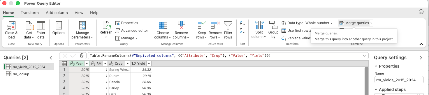
Select the first query (rm_yields_2015_2024) and then click Home > Merge Queries.

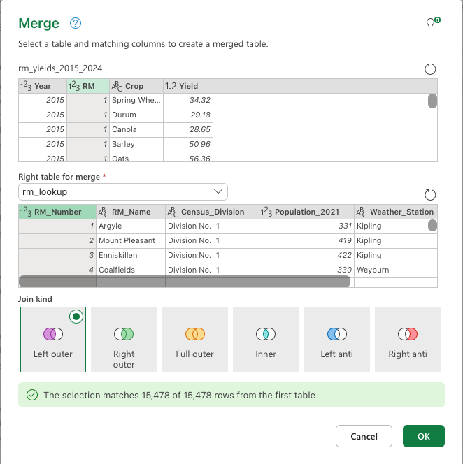
Figure 9.2: The two queries loaded, with the yield data in long format and **Merge queries** on the ribbon.

In the pop up menu (Figure 9.3) select rm_lookup as the right table to merge.
Select the key to merge on in each table by clicking its column heading: RM in the yields table and RM_Number in the lookup table.
Keep Left Outer as the join kind. This keeps every yield observation and adds information wherever the lookup contains a matching RM.
Check the number of matching rows reported at the bottom of the dialog – here every one of the 15,478 yield observations finds a match – then choose OK.

Figure 9.3: The Merge dialog: the two tables, the key selected in each, the join kind, and the match count along the bottom.

The merged data arrives packed into a single new column whose every entry reads [Table] (Figure 9.4). Expand it using the double-arrow icon in its header: tick the columns you want (the RM name, census division, population and closest weather station) and untick Use original column name as prefix so the columns keep their own names.

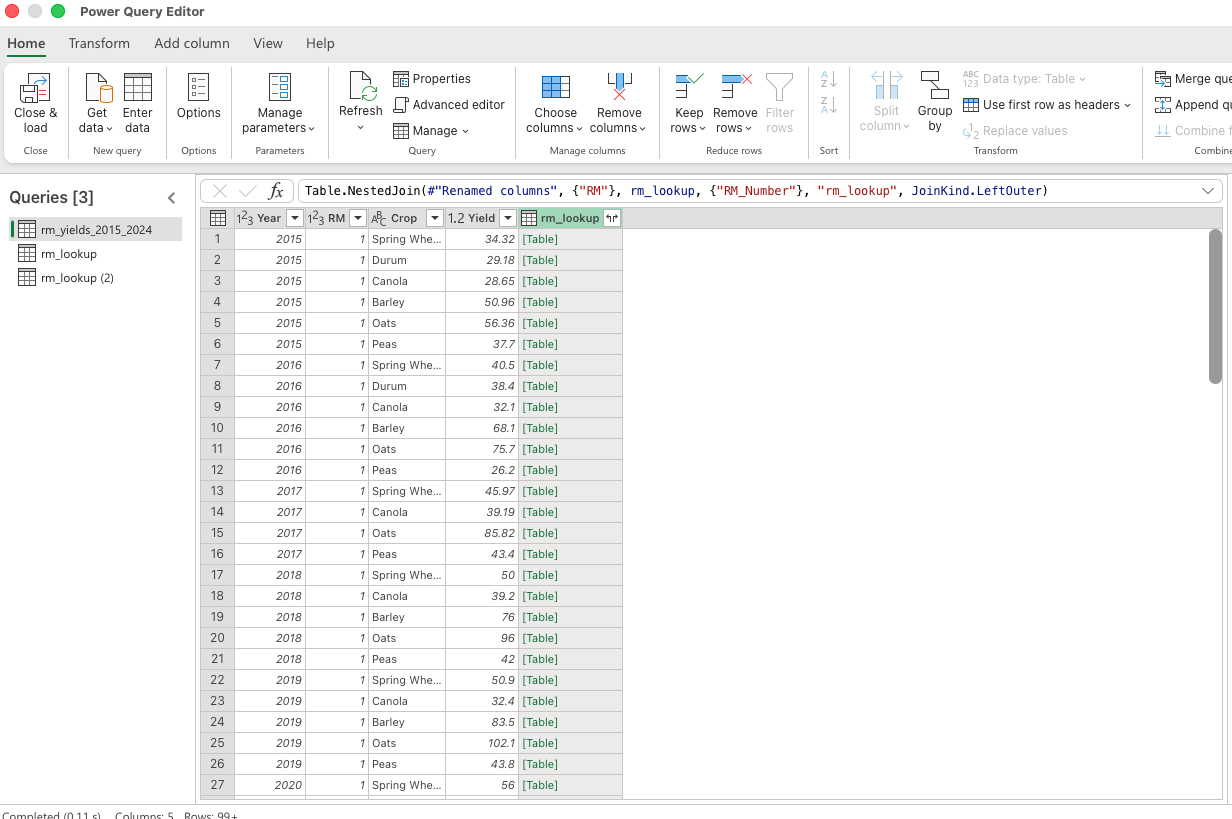
Figure 9.4: After the merge, the lookup columns sit folded inside a `[Table]` column. The double-arrow icon in its header expands them. Do not click a `[Table]` link itself – that drills into that one row’s table and discards the rest.

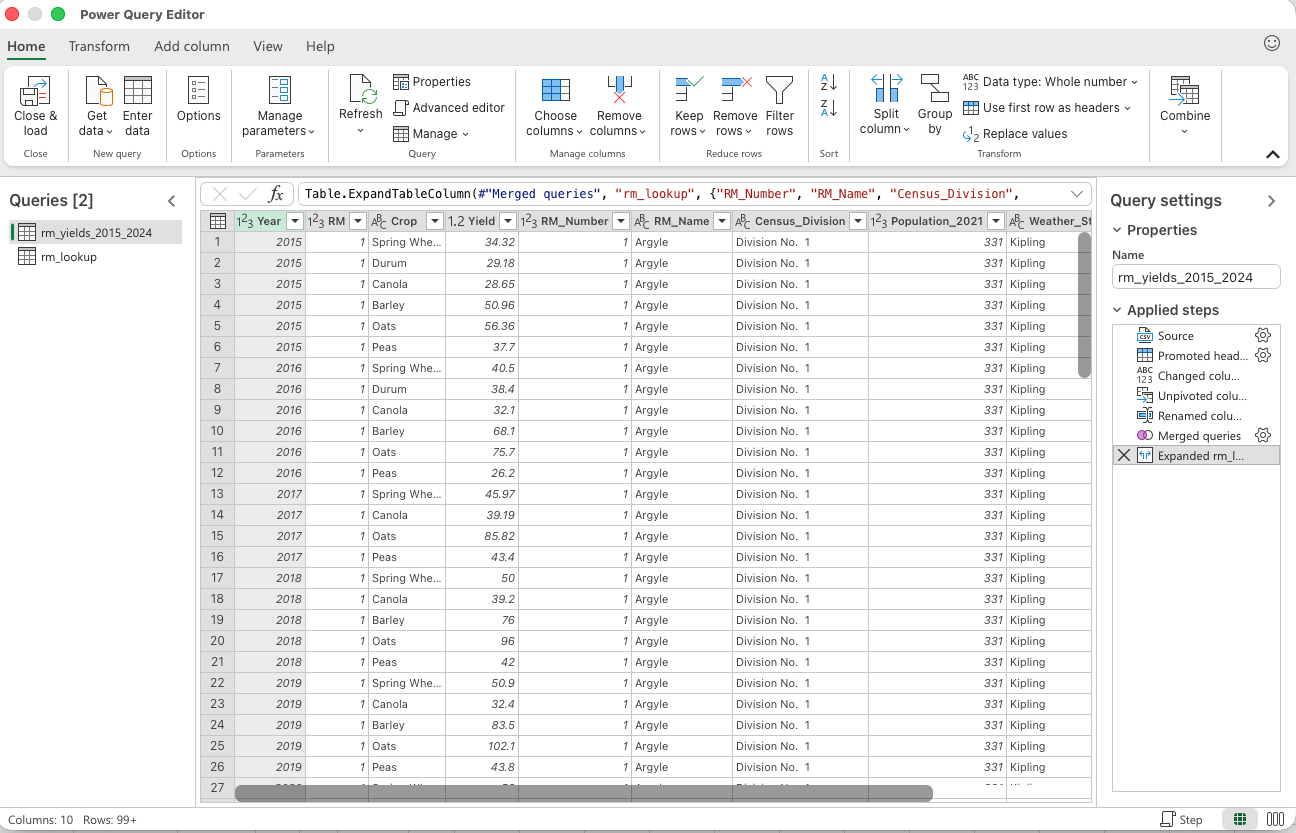
Figure 9.5: After expanding: the lookup columns sit beside every yield observation, and the row count has not changed.

Now you should see the RM lookup data merged with the RM yield data. We can now repeat the same process to merge once again with the station data: import station_precip.csv the same way, so a third query appears (Figure 9.6). The only difference is that we are now going to merge on both the station name and the year (Figure 9.7). Select Weather_Station and then Ctrl-click (Cmd-click on a Mac) Year in the top table, and Station then Ctrl-click Year in the bottom one – the small 1 and 2 beside the headings show the matching order.

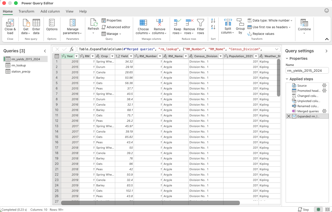
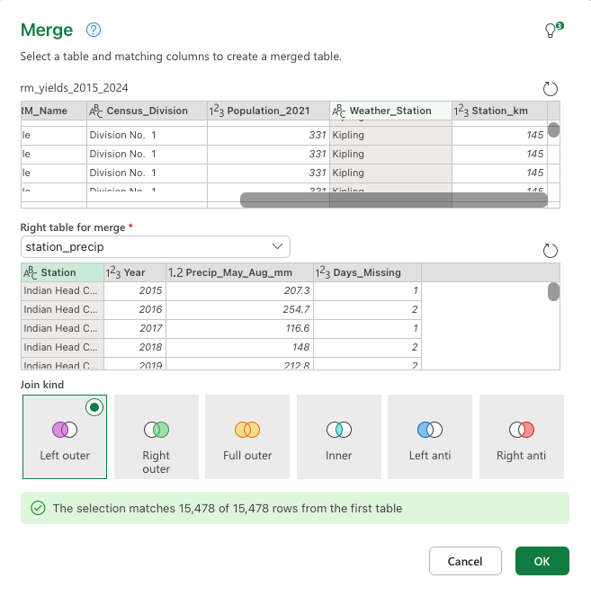
Figure 9.6: The station precipitation data imported as a third query.

Figure 9.7: The second Merge dialog, with the station column selected in each table; Ctrl-clicking `Year` in each adds it as the second key. Station and year together identify the right precipitation value.

After expanding the precipitation column and choosing Close & load, every yield observation carries its RM’s name, closest station, and that station’s growing-season precipitation for the right year.

Download the finished merge workbook – the three queries with their Applied Steps intact.

Checking the merge

After each merge, compare the number of rows with the original yields table. A many-to-one left merge should retain the same number of rows. Filter the expanded columns for null to find observations that did not match, and check several rows against the source tables.

Power Query also offers Inner, Full Outer and Left Anti joins. These correspond to the R joins introduced below. A Left Anti join is particularly useful for listing rows that have no match before completing the merge.

9.2 Merging in R

Video walkthrough of this section

In tidyverse we merge data with join functions. There are four different types of joins depending on which data we want to keep in the merged file. Suppose we have two datasets x and y:

left_join(x, y, by) keeps every row of x whether it has a match in y or not. But does not keep rows in y that don’t have a match.
inner_join(x, y, by) keeps only rows that matched in both tables.
full_join(x, y, by) keeps every row from both tables, regardless of whether there is a match.
anti_join(x, y, by) returns the rows of x that have no match in y. It is useful for finding failed matches before a join.

The by argument specifies the key we merge on, written with join_by(). A column with the same name in both tables is written once, join_by(year); if the key has different names in the two tables, write join_by(left_name == right_name).

The full R code for merging the datasets in R is below. We first read in the three datasets, pivoting the yields to be in long format. We then merge the yield data with the RM lookup using a left join. This keeps all the data in yield data regardless of whether there is a match in the RM lookup, but would not keep any RM lookup rows that do not have a match in the yield data. The exact code for that join is

with_station <- yields_long |>
  left_join(rm_lookup,
            by = join_by(rm == rm_number))

We can read this as set with_station equal to the result of:

Take yields long then
Left join it with the RM lookup.
Merge the dataset by matching rm in the yields_long with rm_number in the RM lookup.

As an exercise, you should see how and why the merge would be different if we used an inner join or full join instead of a left join. Because there is one RM in the rm_lookup that is not in the yields_long, full join will result in more rows – these additional rows will have empty data for columns that are in yields_long. However, because all rows in yields_long have a match in rm_lookup, inner_join will result in the exact same table as left_join – note that this is only because all the RMs in our yield data are represented in the RM lookup data.

We then check the number of rows before and after the merge.

Finally, we merge the with_station dataset with the precipitation data using another left join.

#########################
##### Load packages
#########################

library(tidyverse)
library(janitor)

#########################
##### Step 1: Read in data 
#########################

# Read the yield data and pivot longer
yields <- read_csv("data/rm_yields_2015_2024.csv") |>
  clean_names()      # Year and RM to year and rm; crop columns to snake case

# Pivot yields longer
yields_long <- yields |>
  pivot_longer(
    cols = spring_wheat:peas,      # the six crop columns
    names_to = "crop",
    values_to = "yield_bu_ac"
  )

# Read the RM lookup data
rm_lookup <- read_csv("data/rm_lookup.csv") |>
  clean_names()      # RM_Number becomes rm_number, and so on

# Read the station data 
precip <- read_csv("data/station_precip.csv") |>
  clean_names()      # Station becomes station


#########################
##### Step 2: Merge yields and RM data
#########################

# Add the RM information and nearest station
with_station <- yields_long |>
  left_join(rm_lookup,
            by = join_by(rm == rm_number))

# Print column names to check merge
names(with_station)

# Row counts before and after
nrow(yields_long)
nrow(with_station)

#########################
##### Step 3: Merge in the weather station data
#########################

merged <- with_station |>
  left_join(precip,
            by = join_by(weather_station == station, year))

# Print column names to check merge
names(merged)

# Row counts before and after
nrow(with_station)
nrow(merged)

# Glimpse the merged data frame to check the columns and types
glimpse(merged)

> #########################
> ##### Load packages
> #########################
> 
> library(tidyverse)
── Attaching core tidyverse packages ──────────────────────── tidyverse 2.0.0 ──
✔ dplyr     1.2.1     ✔ readr     2.2.0
✔ forcats   1.0.1     ✔ stringr   1.6.0
✔ ggplot2   4.0.3     ✔ tibble    3.3.1
✔ lubridate 1.9.5     ✔ tidyr     1.3.2
✔ purrr     1.2.2     
── Conflicts ────────────────────────────────────────── tidyverse_conflicts() ──
✖ dplyr::filter() masks stats::filter()
✖ dplyr::lag()    masks stats::lag()
ℹ Use the conflicted package (<http://conflicted.r-lib.org/>) to force all conflicts to become errors
> library(janitor)

Attaching package: 'janitor'
The following objects are masked from 'package:stats':

    chisq.test, fisher.test
> 
> #########################
> ##### Step 1: Read in data 
> #########################
> 
> # Read the yield data and pivot longer
> yields <- read_csv("data/rm_yields_2015_2024.csv") |>
+   clean_names()      # Year and RM to year and rm; crop columns to snake case
Rows: 2950 Columns: 8
── Column specification ────────────────────────────────────────────────────────
Delimiter: ","
dbl (8): Year, RM, Spring Wheat, Durum, Canola, Barley, Oats, Peas

ℹ Use `spec()` to retrieve the full column specification for this data.
ℹ Specify the column types or set `show_col_types = FALSE` to quiet this message.
> 
> # Pivot yields longer
> yields_long <- yields |>
+   pivot_longer(
+     cols = spring_wheat:peas,      # the six crop columns
+     names_to = "crop",
+     values_to = "yield_bu_ac"
+   )
> 
> # Read the RM lookup data
> rm_lookup <- read_csv("data/rm_lookup.csv") |>
+   clean_names()      # RM_Number becomes rm_number, and so on
Rows: 296 Columns: 6
── Column specification ────────────────────────────────────────────────────────
Delimiter: ","
chr (3): RM_Name, Census_Division, Weather_Station
dbl (3): RM_Number, Population_2021, Station_km

ℹ Use `spec()` to retrieve the full column specification for this data.
ℹ Specify the column types or set `show_col_types = FALSE` to quiet this message.
> 
> # Read the station data 
> precip <- read_csv("data/station_precip.csv") |>
+   clean_names()      # Station becomes station
Rows: 160 Columns: 4
── Column specification ────────────────────────────────────────────────────────
Delimiter: ","
chr (1): Station
dbl (3): Year, Precip_May_Aug_mm, Days_Missing

ℹ Use `spec()` to retrieve the full column specification for this data.
ℹ Specify the column types or set `show_col_types = FALSE` to quiet this message.
> 
> 
> #########################
> ##### Step 2: Merge yields and RM data
> #########################
> 
> # Add the RM information and nearest station
> with_station <- yields_long |>
+   left_join(rm_lookup,
+             by = join_by(rm == rm_number))
> 
> # Print column names to check merge
> names(with_station)
[1] "year"            "rm"              "crop"            "yield_bu_ac"    
[5] "rm_name"         "census_division" "population_2021" "weather_station"
[9] "station_km"     
> 
> # Row counts before and after
> nrow(yields_long)
[1] 17700
> nrow(with_station)
[1] 17700
> 
> #########################
> ##### Step 3: Merge in the weather station data
> #########################
> 
> merged <- with_station |>
+   left_join(precip,
+             by = join_by(weather_station == station, year))
> 
> # Print column names to check merge
> names(merged)
 [1] "year"              "rm"                "crop"             
 [4] "yield_bu_ac"       "rm_name"           "census_division"  
 [7] "population_2021"   "weather_station"   "station_km"       
[10] "precip_may_aug_mm" "days_missing"     
> 
> # Row counts before and after
> nrow(with_station)
[1] 17700
> nrow(merged)
[1] 17700
> 
> # Glimpse the merged data frame to check the columns and types
> glimpse(merged) 
Rows: 17,700
Columns: 11
$ year              <dbl> 2015, 2015, 2015, 2015, 2015, 2015, 2016, 2016, 2016…
$ rm                <dbl> 1, 1, 1, 1, 1, 1, 1, 1, 1, 1, 1, 1, 1, 1, 1, 1, 1, 1…
$ crop              <chr> "spring_wheat", "durum", "canola", "barley", "oats",…
$ yield_bu_ac       <dbl> 34.32, 29.18, 28.65, 50.96, 56.36, 37.70, 40.50, 38.…
$ rm_name           <chr> "Argyle", "Argyle", "Argyle", "Argyle", "Argyle", "A…
$ census_division   <chr> "Division No.  1", "Division No.  1", "Division No. …
$ population_2021   <dbl> 331, 331, 331, 331, 331, 331, 331, 331, 331, 331, 33…
$ weather_station   <chr> "Kipling", "Kipling", "Kipling", "Kipling", "Kipling…
$ station_km        <dbl> 145, 145, 145, 145, 145, 145, 145, 145, 145, 145, 14…
$ precip_may_aug_mm <dbl> 183.2, 183.2, 183.2, 183.2, 183.2, 183.2, 313.0, 313…
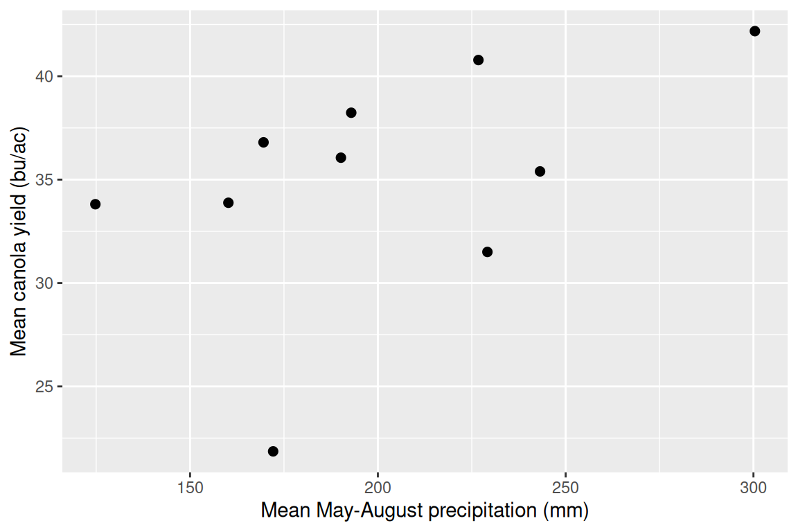
$ days_missing      <dbl> 2, 2, 2, 2, 2, 2, 0, 0, 0, 0, 0, 0, 0, 0, 0, 0, 0, 0…

This data frame would allow us to do further analysis on the relationship between precipitation and yield. We will do that in the later chapters. To give you a preview of this, here is a scatter plot of the mean canola yield and mean precipitation for each year – the correlation is about 0.47.