5 Loading Data and Packages in R

Video walkthrough of this chapter

In the last chapter, we created small datasets directly in R. Real data analysis usually starts with a file. That creates a few practical questions. Where should the file go? How does R find it? How do we bring it into R? And once it is there, how do we check that R has read it correctly?

This chapter develops a simple workflow for working with real data: keep everything for an analysis in one project folder, refer to files with relative paths, use packages to add functions to R, read the data from a CSV file, and inspect it before doing any analysis. These habits are not exciting, but they prevent a remarkable number of problems later.

The data we will work with is a small .csv file of canola yield trials (hypothetical data): 120 fields, each with an ID, a fertilizer rate, growing-season rainfall, a variety, and a yield. It can be downloaded here: canola_trial.csv.

5.1 Setting up a project folder

The temptation after downloading the csv file is to get it loaded into R as quickly as possible. However, it is worth taking a minute (and it only takes less than a minute!) to set up a project folder. The folder will eventually hold your data, code, and output. For complex projects, it would be best to separate these into subfolders. A typical project might look like this:

canola_yields/
  data/
    canola_trial.csv          
  code/
    1_clean.R
    2_analysis.R
  output/
    yield_by_variety.png
    summary_table.csv
  README.md

data/ contains the original data;
code/ contains the scripts, numbered in the order they run;
output/ contains tables, figures, and other results the scripts produce; and
README.md holds notes explaining the project. This becomes more important when we start using AI tools.

The exact folder names matter less than the principle: the project is self-contained. If you zip canola_yields/ and send it to somebody else, they have everything they need to run your analysis.

You can create all this in Positron by selecting File → New Folder from Template…. After you create the folder you will see a file explorer tab open on the left pane of Positron. When you save data or files in your folder you will see them appear in this tab. You can also add new subfolders and files in this pane by either right-clicking in the pane or using the new-folder button.

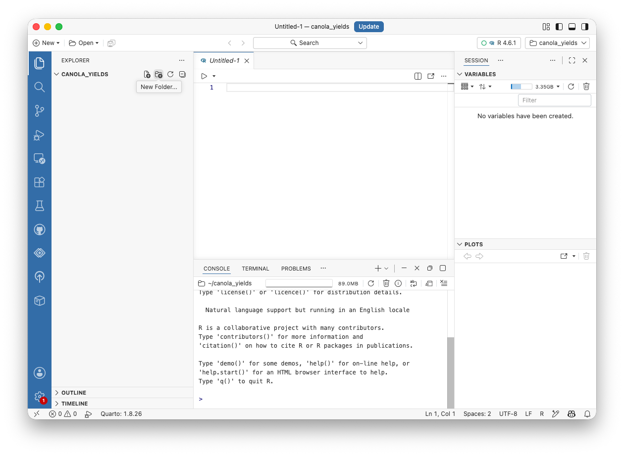
Figure 5.1: The Explorer pane after creating and opening the project folder. The new-folder button (shown with its tooltip) adds subfolders like `data/`, `code/`, and `output/`.

Creating a project folder is important for two reasons. First, it allows you to read in data using relative paths (discussed in Section 5.4). Second, when using AI tools you can choose to provide them access to your whole folder, and they can read all the files and data within that folder to get the context for your entire project (discussed in Module 5).

An alternative set-up you might want for this class is to have an AREC_261 folder with subfolders branching off from there. For example:

AREC_261/
  code/
    module_1/
    module_2/
  data/
  output/
    module_1/
    module_2/
  README.md

Note that I have subfolders for each module in the code/ and output/ folders. But since the datasets we use will be shared across modules, I have just one data/ folder. Others might prefer a different structure.

A final note: Never overwrite your raw data. Suppose canola_trial.csv contains an obvious typo. You could open the file in Excel, fix the cell, and save – but then there is no record of what you changed. Keep the original file exactly as it arrived and make the correction in your R script, where it leaves a trail: what changed, and how.

5.2 Packages

R comes with hundreds of useful built-in functions (like mean() and sd()). However, one of the benefits of R is that other people have written thousands of other functions and bundled them into packages. When you install and load these packages you can use these functions. The first package that we will install is called tidyverse. Using a package is a two-step process:

Install it – once per computer. This downloads the package from the internet and saves it on your machine:
```
install.packages("tidyverse")
```
The first installation can take a few minutes and prints a lot of messages. Some appear in red even when nothing has gone wrong; what matters is whether R ultimately reports an error.
Load it – once per script. Installing puts the package on your computer, but it is not switched on until you load it. Put this at the top of every script that uses the tidyverse:
```
library(tidyverse)
```

If you skip the library() step and try to use a package function, R will stop with an error like:

Error in read_csv(...) : could not find function "read_csv"

That “could not find function” message almost always means you forgot to load the package (or you have not installed it yet). The fix is to run library(tidyverse) first. Note the quirk: you put quotes around the name when you install (install.packages("tidyverse")) but not when you load (library(tidyverse)).

5.3 The Tidyverse

So what is this tidyverse package? It is actually a collection of packages that do different jobs. The four that will matter most in this book are:

Package	Main job
`readr`	reading data
`dplyr`	manipulating data
`tidyr`	reshaping data
`ggplot2`	making graphs

Installing the tidyverse installs these and several others, and library(tidyverse) loads the core packages at once.

Other resources — packages and the tidyverse

R for Data Science (2nd ed.) – the Introduction describes the tidyverse workflow (import → tidy → transform → visualize → model → communicate) this course follows.
tidyverse.org – the package index lists the core packages and what each does.

5.4 Reading Data from CSV

Assuming you have saved the csv file in your project’s data/ folder, you can click on it in Positron’s Explorer pane and the data appears as a spreadsheet. You can use this spreadsheet to get an understanding of the data. Clicking the arrow beside a variable opens a quick histogram of it, along with some summary statistics.

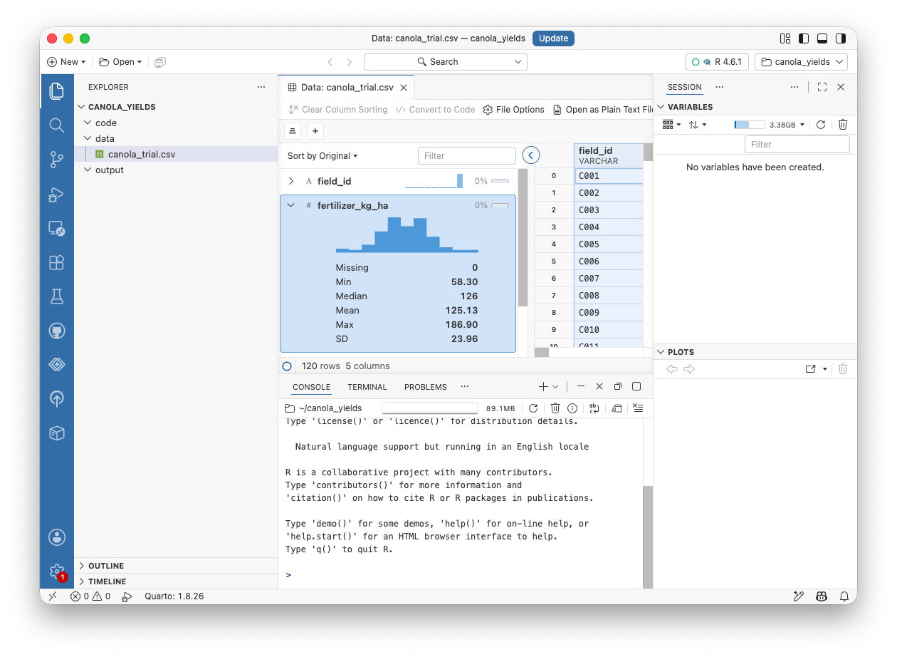
Figure 5.2: Positron’s data viewer on `canola_trial.csv`. Expanding a variable shows its histogram and summary statistics – here `fertilizer_kg_ha`, across the 120 rows.

But note that this data is not yet loaded into R; this is just Positron’s spreadsheet functionality. To actually load the data in R we can create a new script (perhaps calling it code/1_canola_trial_script.R). We can then use the read_csv() function to read in the data and assign it to trial_data. Here is my small script for doing this, and beneath it the console output from running it:

# ---
# Title: Canola trial data
# Author: Your Name
# Date: 2026-09-29
# Description:
#   Reads in the canola trial data and summarizes the
#   variables in the data.
# ---

# Load packages
library(tidyverse)

# Read in the data
trial_data <- read_csv("data/canola_trial.csv")

> trial_data <- read_csv("data/canola_trial.csv")
Rows: 120 Columns: 5
── Column specification ────────────────────────────────────────────────────────
Delimiter: ","
chr (2): field_id, variety
dbl (3): fertilizer_kg_ha, rainfall_mm, yield_bu_acre

ℹ Use `spec()` to retrieve the full column specification for this data.
ℹ Specify the column types or set `show_col_types = FALSE` to quiet this message.

The output is read_csv()’s note about what it just read.

Note that I am using the path data/canola_trial.csv because I created a subfolder called data/ and stored my .csv file in this subfolder. If you didn’t do this or if you created a differently named subfolder then your path will be different. For example, if your folder structure looks like:

AREC_261/
  module_1/
    data/
      canola_data.csv
  README.md

Then your code should read: trial_data <- read_csv("module_1/data/canola_trial.csv"). When you use a project folder you only need to specify the path relative to the project folder (called the relative path). For example, on my computer the full or absolute path for this file is /Users/peter/Documents/canola_yields/data/canola_trial.csv. But because my project folder is canola_yields I only need to specify the part of the absolute path that comes after the folder. The nice part of this convention is that if I share this folder with anyone else, then the paths will all work on their computer too.

One should also note that if we just read in the data but don’t assign it to trial_data – for example if we just run:

read_csv("data/canola_trial.csv")

– then R prints the data to the console but does not save it anywhere. This is the same displaying-versus-saving distinction from the last chapter: without the assignment, there is no object to work with afterwards.

Windows note

Windows displays paths with backslashes, as in C:\Users\Peter\Documents, but a backslash means something special inside an R string. Write forward slashes even on Windows: "C:/Users/Peter/Documents". R handles the translation.

File names

Use short descriptive names without spaces or punctuation: yield_data_final.csv, not Field Yields FINAL!!.csv.

5.5 Inspecting the Data

Successfully reading a file does not mean you are ready to analyze it. Inspect it first:

trial_data              # prints the data frame (first 10 rows)

nrow(trial_data)        # number of rows

ncol(trial_data)        # number of columns

names(trial_data)       # column names

glimpse(trial_data)     # compact column-by-column view, with types

summary(trial_data)     # quick summary of every column

> trial_data              # prints the data frame (first 10 rows)
# A tibble: 120 × 5
   field_id fertilizer_kg_ha rainfall_mm variety    yield_bu_acre
   <chr>               <dbl>       <dbl> <chr>              <dbl>
 1 C001                146.         199. InVigor             56.7
 2 C002                136.         282. DEKALB              62  
 3 C003                113.         274. Clearfield          53.6
 4 C004                112.         173  InVigor             51.2
 5 C005                103.         216. InVigor             49.2
 6 C006                140.         151. InVigor             51.2
 7 C007                102          217  Clearfield          49  
 8 C008                137.         275. InVigor             56.8
 9 C009                142.         258. InVigor             61  
10 C010                 97.9        210. Clearfield          48.2
# ℹ 110 more rows
> 
> nrow(trial_data)        # number of rows
[1] 120
> 
> ncol(trial_data)        # number of columns
[1] 5
> 
> names(trial_data)       # column names
[1] "field_id"         "fertilizer_kg_ha" "rainfall_mm"      "variety"         
[5] "yield_bu_acre"   
> 
> glimpse(trial_data)     # compact column-by-column view, with types
Rows: 120
Columns: 5
$ field_id         <chr> "C001", "C002", "C003", "C004", "C005", "C006", "C007…
$ fertilizer_kg_ha <dbl> 146.2, 136.5, 113.1, 111.8, 102.6, 140.5, 102.0, 136.…
$ rainfall_mm      <dbl> 198.7, 282.3, 273.6, 173.0, 215.5, 151.1, 217.0, 275.…
$ variety          <chr> "InVigor", "DEKALB", "Clearfield", "InVigor", "InVigo…
$ yield_bu_acre    <dbl> 56.7, 62.0, 53.6, 51.2, 49.2, 51.2, 49.0, 56.8, 61.0,…
> 
> summary(trial_data)     # quick summary of every column
      field_id   fertilizer_kg_ha  rainfall_mm         variety   
 Length   :120   Min.   : 58.3    Min.   :128.9   Length   :120  
 N.unique :120   1st Qu.:110.5    1st Qu.:201.8   N.unique :  3  
 N.blank  :  0   Median :126.0    Median :234.9   N.blank  :  0  
 Min.nchar:  4   Mean   :125.1    Mean   :229.1   Min.nchar:  6  
 Max.nchar:  4   3rd Qu.:141.0    3rd Qu.:258.6   Max.nchar: 10  
                 Max.   :186.9    Max.   :320.8                  
                                  NAs    :3                      
 yield_bu_acre  
 Min.   :39.30  
 1st Qu.:49.52  
 Median :52.55  
 Mean   :53.40  
 3rd Qu.:57.73  
 Max.   :70.40

glimpse() shows each column and its type; summary() reports the min, max, mean, median, and quartiles of every numeric column. The goal is not to run these commands mechanically but to answer some questions:

Did I get the number of observations I expected?
Are the variables I expected actually present?
Did R interpret numeric variables as numbers?
Are the values in plausible ranges?
Are there missing values?

Looking at the data before analyzing it catches many mistakes cheaply.

Other resources — reading data from CSV

R for Data Science (2nd ed.) – Chapter 7, “Data import”: reading files with read_csv(), column types, and common import problems.
readr documentation – the tidyverse readr reference for read_csv() and its relatives.
Working directory & path errors – this chapter from Mastering R Through Errors and Warnings explains getwd() and the “file does not exist” error.
Video – Science Grad School Coach, Read and load CSV files into R – loading a CSV step by step.

5.6 Summary Statistics in R

Once the data are in R, we can calculate the same summary statistics we used in Excel. yield_bu_acre is a column of the data frame trial_data, so we refer to it as trial_data$yield_bu_acre:

mean(trial_data$yield_bu_acre)

median(trial_data$yield_bu_acre)

sd(trial_data$yield_bu_acre)

range(trial_data$yield_bu_acre)                        # returns c(min, max)

quantile(trial_data$yield_bu_acre, c(0.25, 0.5, 0.75)) # percentiles

IQR(trial_data$yield_bu_acre)

> mean(trial_data$yield_bu_acre)
[1] 53.39917
> 
> median(trial_data$yield_bu_acre)
[1] 52.55
> 
> sd(trial_data$yield_bu_acre)
[1] 5.767724
> 
> range(trial_data$yield_bu_acre)                        # returns c(min, max)
[1] 39.3 70.4
> 
> quantile(trial_data$yield_bu_acre, c(0.25, 0.5, 0.75)) # percentiles
   25%    50%    75% 
49.525 52.550 57.725 
> 
> IQR(trial_data$yield_bu_acre)
[1] 8.2

var(), min(), and max() work the same way. The statistical ideas have not changed since Module 1; only the way we ask the computer to calculate them has.

One thing you may have spotted: summary(trial_data) above reports NA's :3 under rainfall_mm – three fields have no rainfall reading. NA is R’s code for a missing value, and calculations involving the rainfall column will behave differently because of them. Missing values, and what to do about them, are covered in Section 8.3.

Other resources — summary statistics in R

Video – Rob Spencer, Descriptive statistics using the summary function – a short walkthrough of summary().
Video – Dr E Research Videos, Basic summary statistics in R – mean, median, standard deviation, and the number summary.

5.7 Full Script

The whole chapter fits in one script – the code/1_canola_trial_script.R we started in Section 5.4, now complete with every inspection and summary statistic from the chapter:

# ---
# Title: Canola trial data
# Author: Your Name
# Date: 2026-09-29
# Description:
#   Reads in the canola trial data and summarizes the
#   variables in the data.
# ---

# Load packages
library(tidyverse)

# Read in the data
trial_data <- read_csv("data/canola_trial.csv")

# Inspect the structure
trial_data           # print the first rows
nrow(trial_data)     # number of rows
ncol(trial_data)     # number of columns
names(trial_data)    # column names
glimpse(trial_data)  # columns, types, and first values

# Inspect the values
summary(trial_data)

# Summary statistics for yield
mean(trial_data$yield_bu_acre)
median(trial_data$yield_bu_acre)
sd(trial_data$yield_bu_acre)
range(trial_data$yield_bu_acre)
quantile(trial_data$yield_bu_acre, c(0.25, 0.5, 0.75))
IQR(trial_data$yield_bu_acre)