1 Getting Started with Excel
This chapter introduces the basic building blocks of Excel. Likely you have already used Excel or another spreadsheet program, such as Google Sheets. If so, much of what we cover in this chapter might be a review. Make sure that you have Excel installed on your computer – the online and mobile versions do not have the same functionality. Your Excel should be licesned under Microsoft 365, which is continually updated and available to students through the University.
1.1 Workbooks and Worksheets
A workbook is one Excel file. Inside it are worksheets – the tabs along the bottom of the window. Many people who start using Excel think in terms of a single worksheet. They put their data, analysis, and charts within that worksheet. This requires you to scroll up and down or left and right to find everythign in the worksheet.
A better approach is to think of a workbook as a collection of worksheets, each performing a different function. For example, we should always keep our raw data in a separate worksheet. Then we might have cleaned data in another worksheet, and our analysis and charts in yet another. This makes it easier to find what you are looking for and to share your workbook with others.
Most of what we will do in this chapter involves small calculations within a single worksheet. We will return to workbook organization in later chapter.
- Excel for Dummies – Microsoft 365 Excel for Dummies, the opening chapters on the Excel interface and workbook basics.
- Microsoft Support – Excel for Windows training, Microsoft’s own free tutorial hub.
- Video (beginner overview) – How to use Excel for beginners – a short tour of entering data, formatting, and the interface.
1.2 File Formats and File Management
In this class, we will read in data in two formats:
.xlsx– The standard modern Excel workbook format. It can contain multiple worksheets, formulas, formatting, charts, and PivotTables. We will generally use this format when we are working in Excel. The older.xlsformat was the standard Excel format before 2007..csv– Comma-separated values. A CSV is a simple text file containing a single table: each line represents a row, with values separated by commas. CSV files contain data only – not formulas, formatting, charts, or multiple worksheets. Because the format is simple and widely supported, CSV is commonly used to store and exchange tabular data between programs such as Excel, R, Python, and other statistical software.
Excel will readily open a .csv file. However, be careful: Excel sometimes tries to be helpful by automatically interpreting the data. For example, it might turn SEPT1 into the date 1-Sep, or remove leading zeros from a farm ID such as 00127. These changes can alter the underlying data. When this might be a problem, use Data → Get Data → From Text/CSV, which lets you inspect and set column types explicitly, rather than simply double-clicking the file.
- Microsoft Support – Import or export text (.txt or .csv) files, including the Text Import Wizard that lets you set column types.
- Microsoft Support – File formats that are supported in Excel, if you meet an unfamiliar extension.
1.3 Cells and Formulas
Each cell in a worksheet has an address formed by its column letter and row number: A1, B2, AA35, and so on. A cell can contain:
- A number:
42,3.14,-1000 - Text:
Canola,Field 7,North field - A date:
2026-09-15(Excel stores dates internally as numbers; we will return to this later.) - A formula: anything starting with
=
A formula is a calculation. It can be as simple as =2+2, but the real power of a spreadsheet comes from formulas that reference other cells. For example, =A2+B2 adds the values in cells A2 and B2.
Because the formula references the cells rather than fixed numbers, it recalculates whenever those cells change. Change the value in A2, and every formula that references A2 updates automatically.
Excel uses the standard mathematical operators – +, -, * (multiply), / (divide), and ^ (exponent) – and it evaluates them in the standard PEMDAS order: Parentheses, Exponents, Multiplication/Division, then Addition/Subtraction, working left to right within each level.
The worksheet below provides examples of simple operations.
Download this workbook · Open online (File → Save a Copy to view formulas and edit)
(If an embedded workbook does not load, use the Open online or Download link instead – neither requires an account.)
- Excel for Dummies – Microsoft 365 Excel for Dummies, the chapter on entering formulas.
- Microsoft Support – Overview of formulas in Excel and Calculation operators and precedence.
- Video (order of operations) – Order of operations for math formulas in Excel.
1.4 Relative and Absolute References
When you write a formula like =A2-B2 in cell C2 and then copy that formula down to C3, Excel automatically changes it to =A3-B3. This is called a relative reference: Excel interprets A2 not just as “cell A2,” but as the cell two columns to the left and in the same row as the formula. When the formula moves, the reference moves with it.
Usually, this is exactly what you want. For example, suppose column A contains sales, column B contains costs, and you want to calculate profit in column C. Each row should subtract that row’s costs from that row’s sales. You can write the formula once and then copy it down the column.
Sometimes, however, you do not want a reference to change. Sheet Abs ref in the work book below shows an example of this – in this worksheet we want to each cell in column C to equal the product of the cell in column C and cell B8 (which holds a conversion factor). If in cell C2 we write =A2*B8 and copy it down, the formula in C3 becomes =A3*B9, which is not what we want.
The fix is to use an absolute reference. A $ locks whatever comes immediately after it. For example:
A1– relative column, relative row (changes when copied in either direction)$A1– absolute column, relative row (column stays as A, row changes)A$1– relative column, absolute row (column changes, row stays as 1)$A$1– absolute column and row (neither changes; “locked”)
In the worksheet below, you would write in C2 =B2*$B$8. When you copy the formula down, B2 becomes B3, A4, and so on, while $B$8 remains $B$8.
Download this workbook
Open online (File → Save a Copy to view formulas and edit). The workbook includes practice sheets to fill in yourself.
- Microsoft Support – Switch between relative, absolute, and mixed references.
- Excel for Dummies – Microsoft 365 Excel for Dummies, the chapter on cell references.
- Video – Excel Relative and Absolute Cell References – what happens to references when you copy a formula, and what the
$signs do.
1.5 Cell Formatting
In the formulas above, we were working only with numbers. Cells can also contain text, dates, and times. Additionally, numbers can be displayed in different ways. Excel uses number formats to control how values appear. Common formats include General, Number, Currency, Percentage, and Date. Excel normally defaults to General, but may automatically apply another format when it recognizes what you enter. For example, entering a date may cause Excel to apply a date format automatically.
Excel gives you one free clue about what it thinks a cell holds. Numbers, dates and times sit against the right edge of their cell by default; text sits against the left. So a column of dates that lines up on the left has been read as text, and will not behave like a date.
You can change the format of a cell by right-clicking on it and choosing Format Cells (Figure 1.1 (a)). This opens a dialog where you can choose a format and adjust options such as the number of decimal places, currency symbol, or how a date is displayed.
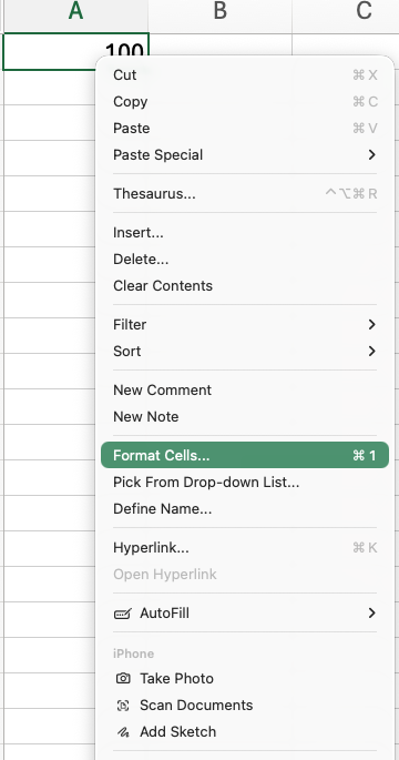
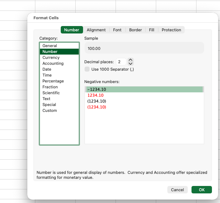
100, but the Number category with two decimal places displays it as 100.00
Two formatting issues are particularly important: decimal places and dates. When presenting numbers, use a level of precision that is meaningful for the audience. For example, reporting an average yield as 40.5 bushels per acre is usually more useful than reporting 40.519834760. Excel lets you control the number of decimal places displayed without changing the underlying value.
Dates require some additional care because Excel can perform calculations with them. For example, if a cell contains September 7, 2027 as a date, adding 7 gives September 14, 2027. If September 7, 2027 is stored as text instead, Excel cannot treat it in the same way.
Importantly, formatting changes how a value looks, not the underlying value Excel uses in calculations. A cell containing 0.45 can be displayed as 45%, and a cell containing 1000 can be displayed as $1,000.00. Formulas that reference those cells still use the underlying values 0.45 and 1000.
The distinction matters when the numbers are added up. Five yields formatted to zero decimals still total their unrounded selves, so a column that reads 41, 39, 45, 36, 40 can show a total of 200.7 – which looks like an arithmetic error to anyone reading it.
Download this workbook
Open online (File → Save a Copy to view formulas and edit). The workbook includes a practice sheet to fill in yourself.
- Microsoft Support – Available number formats in Excel and Format a date the way you want.
- Excel for Dummies – Microsoft 365 Excel for Dummies, the chapter on formatting worksheets.
1.6 Ranges and Functions
Every formula so far has referred to cells one at a time – for example, =A2*B2 or =B7*$B$4. That works when you are combining a few numbers, but it quickly becomes impractical. If you have 500 fields and want to calculate their total acres, you are not going to write =A2+A3+A4+... for 500 rows.
Instead, Excel lets you refer to a whole block of cells at once. This block is called a range, and it is written using two corner cells separated by a colon:
B2:B6is the five cells running down column B from row 2 to row 6.B2:D2is the three cells running across row 2 from column B to column D.B5:D9is the rectangle withB5in the top left andD9in the bottom right – fifteen cells in all.
Many Excel functions take a range as their input. A function is a built-in formula that performs a specific calculation. Functions typically require at least one argument. Common functions include:
=SUM(B2:B6)adds the values in the range.=AVERAGE(B2:B6)returns their mean.=COUNT(B2:B6)returns how many of the cells hold a number.
The worksheet below contains five wheat fields. Column B gives the size of each field in acres, and column C gives its yield in bushels per acre. Multiplying the two gives the total bushels produced by each field. Total acres can then be calculated with =SUM(B2:B6), while total production is =SUM(D2:D6). Column E shows the formula used in each cell of column D so that you can see how the calculations work.
Download this workbook
Open online (File → Save a Copy to view formulas and edit). The workbook includes a practice sheet to fill in yourself.
The rows under the table show all three at work: the total, the average, and the count. =AVERAGE(B2:B6) gives 188 acres – the mean field size – and =COUNT(B2:B6) gives 5.
COUNT is more useful than it first looks, because it counts numbers, not cells. Blank cells and text are skipped, so it tells you how many observations you actually have rather than how big the range is. COUNTA counts every non-empty cell, text included, if that is what you want.
A few more details. You can give any of these functions more than one range by separating them with commas, and you can include individual numbers: =SUM(B2:B6,40) adds 40 acres of summerfallow that are not in the table. A range can also run across a row rather than down a column. But be careful – =SUM(B2:D2) would add acres, yield, and total bushels together. Excel will calculate it without complaint, even though the result means nothing.
The main mistake to watch for is a range that does not include the cells you think it does. If you add three new fields below the table, =SUM(B2:B6) will continue to total only the original five. When you click a cell containing a formula, Excel outlines the range it is using. Check that the highlighted cells match the data you intend to include.
One more thing that comes up constantly: a blank cell is not a zero. AVERAGE, COUNT and MEDIAN skip blanks, which is usually what you want. If you fill the blanks with zeros first, those zeros become real measurements and drag the average down.
- Microsoft Support – SUM function and Use Excel as your calculator.
- Excel for Dummies – Microsoft 365 Excel for Dummies, the chapter on built-in functions.