This bank holds 35 questions: five in each section.
Section 1 covers downloading data in R
Sections 2 and 3 cover data shape in Excel and R
Sections 4 and 5 cover cleaning data in Excel and R
Sections 6 and 7 cover merging data in Excel and R
Each question names the dataset it uses, and the paired Excel and R questions share a file. Most hold about twenty rows; the data-cleaning questions in Sections 4 and 5 are a few hundred rows, because the problems in them do not show up by scrolling. All of them are in one download:
Module 3 bank data (ZIP). Unzip it into your project’s data/ folder so the files sit in data/module03/. Each question also links to its own file. The files describe one farm: twenty named fields, five elevators, five weather stations and the spring wheat varieties grown around Rosetown. Yields are in bu/ac unless a question says otherwise; delivery weights are in tonnes.
Your module test will contain three questions, each drawn from a different section. The datasets you need will be provided in the test.
Each question names its tool on a Tool: line. The bank includes Excel questions answered with Power Query and R questions, and your test will hold a mix of the two. The questions that use the openmeteo and cansim packages have no Excel equivalent, so they are R questions.
Each question is worth 10 marks, and the marks for each part are shown beside it. Presentation is not a separate mark: a part that produces the right answer in an unreadable or unlabelled form does not earn all of its marks.
If you submit an R script, it should have a header block, a clearly labelled section for each question, and your sentence answers written as comments, and it should run from top to bottom in a fresh session. If you submit a workbook, it should have a separate worksheet for each question, clearly labelled with the question number, with the queries still attached so the Applied Steps can be seen. Write sentence answers in worksheet cells rather than cell comments so that they are visible when the workbook is opened. Here is an example of what a test will look like and a script that would earn full marks:
Procedure for test:
At least an hour before the test, “Schedule an appointment” in the test for that day.
Bring your (charged) laptop to the test.
Your test will be accessible at 11:30am.
When you get to the room:
Close all applications other than your webbrowser (used to access the test) and Excel or Positron.
Log into zoom and join the breakout room with your name on it.
In Zoom, share your screen (not an application window, but your whole screen) and record your session.
Navigate to Canvas and access your test.
Download the datasets that you need
Complete the test in Excel or Positron.
Upload the completed script or workbook to Canvas (while still logged into zoom).
Leave zoom, and upload the screenshot recording to Canvas.
Your done!!
Section 1 — Downloading data in R
These questions are about getting data into R from an API, using the openmeteo and cansim packages. Both are demonstrated in Downloading data via an R package. Install them before the test: openmeteo comes from GitHub via remotes, and cansim from CRAN. get_cansim() downloads a large table, so give it time to run.
Question 1
Tool: RThis question uses the openmeteo package. Saskatoon is at latitude 52.13, longitude -106.67.
(a) [6 marks] Download hourly temperatures for Saskatoon for the first week of July 2024 with weather_history(), asking for the hourly variable temperature_2m and the America/Regina timezone.
(b) [4 marks] Report the number of rows returned, the highest temperature in the week, and the mean temperature.
Answer
# (a) Hourly temperature for Saskatoon, 1-7 July 2024library(openmeteo)temps <-weather_history(c(52.13, -106.67),start ="2024-07-01", end ="2024-07-07",hourly ="temperature_2m",timezone ="America/Regina")head(temps)# (b) One row per hour: 7 days x 24 hoursnrow(temps)max(temps$hourly_temperature_2m)mean(temps$hourly_temperature_2m)
> # (a) Hourly temperature for Saskatoon, 1-7 July 2024
> library(openmeteo)
> temps <- weather_history(c(52.13, -106.67),
+                          start = "2024-07-01", end = "2024-07-07",
+                          hourly = "temperature_2m",
+                          timezone = "America/Regina")
Error: Timeout was reached [archive-api.open-meteo.com]:
SSL connection timeout
> head(temps)
Error: object 'temps' not found
>
> # (b) One row per hour: 7 days x 24 hours
> nrow(temps)
Error: object 'temps' not found
> max(temps$hourly_temperature_2m)
Error: object 'temps' not found
> mean(temps$hourly_temperature_2m)
Error: object 'temps' not found
Question 2
Tool: RThis question uses the openmeteo package. Swift Current is at latitude 50.29, longitude -107.79.
(a) [6 marks] Download daily weather for Swift Current for June, July and August 2024, asking for two daily variables at once: temperature_2m_max and precipitation_sum. Use the America/Regina timezone.
(b) [4 marks] Report the total rainfall over the three months and the number of days the maximum temperature was above 30 degrees.
Answer
# (a) Two daily variables in one call, given as a vectorlibrary(openmeteo)summer <-weather_history(c(50.29, -107.79),start ="2024-06-01", end ="2024-08-31",daily =c("temperature_2m_max", "precipitation_sum"),timezone ="America/Regina")head(summer)# (b) Season rainfall and the count of hot dayssum(summer$daily_precipitation_sum)sum(summer$daily_temperature_2m_max >30)
> # (a) Two daily variables in one call, given as a vector
> library(openmeteo)
> summer <- weather_history(c(50.29, -107.79),
+                           start = "2024-06-01", end = "2024-08-31",
+                           daily = c("temperature_2m_max", "precipitation_sum"),
+                           timezone = "America/Regina")
> head(summer)
# A tibble: 6 × 3
  date       daily_temperature_2m_max daily_precipitation_sum
  <date>                        <dbl>                   <dbl>
1 2024-06-01                     20.1                     0
2 2024-06-02                     19.5                     7.2
3 2024-06-03                     20.7                    11.2
4 2024-06-04                     20.5                    14.8
5 2024-06-05                     18.4                     0.1
6 2024-06-06                     19.6                     0
>
> # (b) Season rainfall and the count of hot days
> sum(summer$daily_precipitation_sum)
[1] 145.2
> sum(summer$daily_temperature_2m_max > 30)
[1] 18
Question 3
Tool: RThis question uses the cansim package. Statistics Canada table 32-10-0359-01 holds seeded area, production and yield for field crops by province. The measures sit in Harvest disposition, and the numbers are in VALUE.
(a) [5 marks] Download the table with get_cansim() and report how many rows it has.
(b) [5 marks] Filter to the average yield of all wheat in Saskatchewan, in kilograms per hectare, for 2015 to 2025 (the crop is named Wheat, all in the table). Keep the year and the value.
Answer
# (a) The whole table -- every province, crop, year and dispositionlibrary(cansim)field_crops <-get_cansim("32-10-0359-01")nrow(field_crops)# (b) Saskatchewan wheat yield since 2015sk_wheat <- field_crops |>filter(GEO =="Saskatchewan",`Type of crop`=="Wheat, all",`Harvest disposition`=="Average yield (kilograms per hectare)",as.numeric(REF_DATE) >=2015,as.numeric(REF_DATE) <=2025) |>select(REF_DATE, VALUE)sk_wheat
Tool: RThis question uses the openmeteo package. Rosetown is at latitude 51.55, longitude -108.00.
(a) [6 marks] Download daily precipitation totals for Rosetown for May 2024 with weather_history(), asking for the daily variable precipitation_sum and the America/Regina timezone.
(b) [4 marks] Report total precipitation for the month and the date of the wettest day.
Answer
# (a) Daily precipitation for Rosetown, May 2024library(openmeteo)rain <-weather_history(c(51.55, -108.00),start ="2024-05-01", end ="2024-05-31",daily ="precipitation_sum",timezone ="America/Regina")head(rain)# (b) Monthly total and the wettest daysum(rain$daily_precipitation_sum)rain |>arrange(desc(daily_precipitation_sum)) |>head(1)
> # (a) Daily precipitation for Rosetown, May 2024
> library(openmeteo)
> rain <- weather_history(c(51.55, -108.00),
+                         start = "2024-05-01", end = "2024-05-31",
+                         daily = "precipitation_sum",
+                         timezone = "America/Regina")
> head(rain)
# A tibble: 6 × 2
  date       daily_precipitation_sum
  <date>                       <dbl>
1 2024-05-01                    22
2 2024-05-02                     4.9
3 2024-05-03                     0.1
4 2024-05-04                     2.5
5 2024-05-05                     0
6 2024-05-06                     5.7
>
> # (b) Monthly total and the wettest day
> sum(rain$daily_precipitation_sum)
[1] 82.5
> rain |>
+   arrange(desc(daily_precipitation_sum)) |>
+   head(1)
# A tibble: 1 × 2
  date       daily_precipitation_sum
  <date>                       <dbl>
1 2024-05-01                      22
Question 5
Tool: RThis question uses the cansim package. Statistics Canada table 32-10-0359-01 holds seeded area, production and yield for field crops by province. Crops are named as in the table (Canola (rapeseed), Lentils) and the measures sit in Harvest disposition.
(a) [4 marks] Download the table with get_cansim().
(b) [6 marks] Filter to Saskatchewan canola production in metric tonnes for 2020 to 2025 and keep the year and value.
Answer
# (a) Download the whole tablelibrary(cansim)field_crops <-get_cansim("32-10-0359-01")# (b) Saskatchewan canola production since 2020sk_canola <- field_crops |>filter(GEO =="Saskatchewan",`Type of crop`=="Canola (rapeseed)",`Harvest disposition`=="Production (metric tonnes)",as.numeric(REF_DATE) >=2020,as.numeric(REF_DATE) <=2025) |>select(REF_DATE, VALUE)sk_canola
These questions are about making a wide table long in Power Query with Unpivot Columns and Unpivot Other Columns, and saying what one row represents in each shape. Note that Unpivot drops blank cells. The summarizing steps use the conditional functions and PivotTables from Module 1.
Question 6
Tool: Excel (Power Query)The file q06_field_crops_wide.csv has one row per field and one column per crop, holding yields in bu/ac, with blanks where a field did not grow that crop.
(a) [6 marks] Import the file and make the table long with Unpivot Other Columns, so that one column holds the crop and another holds the yield. Report the row count.
(b) [4 marks] Use AVERAGEIF to compute the mean yield of canola.
Tool: Excel (Power Query)The file q07_prices_wide.csv has one row per crop and one column per elevator, holding the price offered in dollars per bushel.
(a) [6 marks] Import the file and make the table long, with an elevator column and a price_per_bu column.
(b) [4 marks] Insert a PivotTable with crop in the rows, elevator in the columns, and the mean price in the values. Turn on the row and column grand totals so the table also shows the mean price for each crop and for each elevator.
Tool: Excel (Power Query)The file q08_farm_fields_wide.csv has one row per farm, field and year, with four crop columns of yields in bu/ac and blanks where a crop was not grown.
(a) [6 marks] Import the file and make the table long, with a column for crops and another for yields.
(b) [4 marks] Filter the long table to canola fields in 2025.
Tool: Excel (Power Query)The file q09_expenses_wide.csv is an operating expense summary: one row per farm, and one column for each expense category, in dollars. A blank means nothing was spent on that category.
(a) [6 marks] Import the file and make the table long, so that one column holds the category and another holds the amount.
(b) [4 marks] Build a PivotTable on the long table showing the total spent in each category.
The same work in R, with pivot_longer() to go long and pivot_wider() to go wide. Note the one difference between the tools: Unpivot drops blank cells, while pivot_longer() keeps them as NA unless you add values_drop_na = TRUE.
Question 11
Tool: RThe file q06_field_crops_wide.csv has one row per field and one column per crop, holding yields in bu/ac, with blanks where a field did not grow that crop.
(a) [6 marks] Read the file and make it long with pivot_longer(), so that one column holds the crop and another holds the yield. Report the row count.
(b) [4 marks] Compute the mean yield of canola.
Answer
library(tidyverse)# (a) one row per field-cropcrops <-read_csv("data/module03/q06_field_crops_wide.csv", show_col_types =FALSE) |>pivot_longer(cols =-field, names_to ="crop", values_to ="yield_bu_ac",values_drop_na =TRUE)nrow(crops)# (b) mean canola yieldcrops |>filter(crop =="Canola") |>summarise(mean_yield =mean(yield_bu_ac))
Tool: RThe file q07_prices_wide.csv has one row per crop and one column per elevator, holding the price offered in dollars per bushel.
(a) [6 marks] Read the file and make it long, with an elevator column and a price_per_bu column.
(b) [4 marks] Compute the mean price for each crop and for each elevator.
Answer
library(tidyverse)# (a) one row per crop-elevatorprices <-read_csv("data/module03/q07_prices_wide.csv", show_col_types =FALSE) |>pivot_longer(cols =-crop, names_to ="elevator", values_to ="price_per_bu")prices# (b) the two summariesprices |>group_by(crop) |>summarise(mean_price =mean(price_per_bu))prices |>group_by(elevator) |>summarise(mean_price =mean(price_per_bu))
> library(tidyverse)
>
> # (a) one row per crop-elevator
> prices <- read_csv("data/module03/q07_prices_wide.csv", show_col_types = FALSE) |>
+   pivot_longer(cols = -crop, names_to = "elevator", values_to = "price_per_bu")
> prices
# A tibble: 30 × 3
   crop         elevator   price_per_bu
   <chr>        <chr>             <dbl>
 1 Canola       Rosetown          13.7
 2 Canola       Kindersley        14.4
 3 Canola       Davidson          13.6
 4 Canola       Outlook           14.4
 5 Canola       Biggar            15.0
 6 Spring Wheat Rosetown           7.77
 7 Spring Wheat Kindersley         8.02
 8 Spring Wheat Davidson           8.43
 9 Spring Wheat Outlook            7.72
10 Spring Wheat Biggar             7.87
# ℹ 20 more rows
>
> # (b) the two summaries
> prices |> group_by(crop) |> summarise(mean_price = mean(price_per_bu))
# A tibble: 6 × 2
  crop         mean_price
  <chr>             <dbl>
1 Barley             5.33
2 Canola            14.2
3 Durum              9.15
4 Oats               4.58
5 Peas              10.6
6 Spring Wheat       7.96
> prices |> group_by(elevator) |> summarise(mean_price = mean(price_per_bu))
# A tibble: 5 × 2
  elevator   mean_price
  <chr>           <dbl>
1 Biggar           8.84
2 Davidson         8.60
3 Kindersley       8.66
4 Outlook          8.55
5 Rosetown         8.55
Question 13
Tool: RThe file q08_farm_fields_wide.csv has one row per farm, field and year, with four crop columns of yields in bu/ac and blanks where a crop was not grown.
(a) [6 marks] Read the file and make it long, with a column for crops and another for yields.
(b) [4 marks] Filter the long table to canola fields in 2025.
Answer
library(tidyverse)# (a) one row per farm-field-year-cropfields <-read_csv("data/module03/q08_farm_fields_wide.csv", show_col_types =FALSE) |>pivot_longer(cols =-c(farm, field, year), names_to ="crop",values_to ="yield_bu_ac", values_drop_na =TRUE)nrow(fields)# (b) canola in 2025fields |>filter(crop =="Canola", year ==2025)
Tool: RThe file q09_expenses_wide.csv is an operating expense summary: one row per farm, and one column for each expense category, in dollars. A blank means nothing was spent on that category.
(a) [6 marks] Read the file and make it long, so that one column holds the category and another holds the amount.
(b) [4 marks] Compute the total spent in each category.
Answer
library(tidyverse)# (a) one row per farm-categoryexpenses <-read_csv("data/module03/q09_expenses_wide.csv", show_col_types =FALSE) |>pivot_longer(cols =-farm, names_to ="category", values_to ="amount",values_drop_na =TRUE)nrow(expenses)# (b) total by categoryexpenses |>group_by(category) |>summarise(total =sum(amount)) |>arrange(desc(total))
Tool: RThe file q15_field_crops_long.csv is long: one row per field and crop, holding the yield in bu/ac. Not every field grew every crop.
(a) [6 marks] Use pivot_wider() to give each crop its own column, with one row per field. Report the number of rows and columns before and after.
(b) [4 marks] Compute the mean canola yield from the wide table (ignore fields that did not grow canola – that is those with NA values).
Answer
# (a) One row per field, one column per croplong <-read_csv("data/module03/q15_field_crops_long.csv", show_col_types =FALSE)dim(long)wide <- long |>pivot_wider(names_from = crop, values_from = yield_bu_ac)dim(wide)wide# (b) Mean canola yield over the fields that grew itmean(wide$Canola, na.rm =TRUE)
> # (a) One row per field, one column per crop
> long <- read_csv("data/module03/q15_field_crops_long.csv", show_col_types = FALSE)
> dim(long)
[1] 25  3
> wide <- long |>
+   pivot_wider(names_from = crop, values_from = yield_bu_ac)
> dim(wide)
[1] 8 5
> wide
# A tibble: 8 × 5
  field       Peas `Spring Wheat` Canola Barley
  <chr>      <dbl>          <dbl>  <dbl>  <dbl>
1 Home        32.4           58.8   37     85.8
2 Kestrel     NA             47.9   NA     56.5
3 Meadowvale  57.2           NA     NA     79.9
4 Nightjar    35.7           62     NA     85
5 Rented      37.7           71.8   45.9   72
6 Coulee      32.9           69.7   32.4   66.9
7 Ridge       52.5           46.1   37.4   56.8
8 Slough      33.1           NA     43.9   NA
>
> # (b) Mean canola yield over the fields that grew it
> mean(wide$Canola, na.rm = TRUE)
[1] 39.32
Section 4 — Data cleaning in Excel
Each of these gives you a file of a few hundred rows with at most three columns, and one or two things wrong with it. Use summary statistics and a histogram to find the problem, then fix it in Power Query and recompute.
Question 16
Tool: Excel (Power Query)The file q16_yield_sentinel.csv has one row per field, with the crop and the recorded yield in bu/ac, for 280 fields.
(a) [4 marks] Import the file and report the minimum, mean and maximum of yield_bu_ac, and make a histogram of it.
(b) [3 marks] Something in this column is wrong. Say what it is, and which statistic shows it.
(c) [3 marks] Load the data through Power Query, correcting the problem you identified in part (b), then recompute the three statistics.
Answer
(b) The minimum is -99, which is not a yield. The office records a field that was never harvested as -99 rather than leaving it blank, and averaging over those rows drags the mean down.
Tool: Excel (Power Query)The file q17_yield_units.csv has one row per field and the spring wheat yield recorded for it. The column is labelled bu/ac. It covers 260 fields. A bushel of wheat weighs 60 lb.
(a) [4 marks] Import the file and report the minimum, mean and maximum of yield_bu_ac, and make a histogram of it.
(b) [3 marks] Something in this column is wrong. Say what it is, and which statistic shows it.
(c) [3 marks] Load the data through Power Query, correcting the problem you identified in part (b), then recompute the three statistics on the corrected column.
Answer
(b) The maximum is in the thousands, far above any real bushel-per-acre yield. Some rows were recorded in lb/ac instead, so one column holds two units.
Tool: Excel (Power Query)The file q18_moisture_decimal.csv holds one row per delivery ticket, with the date and the moisture reading as a percentage. It covers 240 tickets.
(a) [4 marks] Import the file and report the minimum, mean and maximum of moisture_pct, and make a histogram of it.
(b) [3 marks] Something in this column is wrong. Say what it is, and which statistic shows it.
(c) [3 marks] Load the data through Power Query, correcting the problem you identified in part (b), then recompute the three statistics.
Answer
(b) The maximum is over 100, which is impossible for a moisture percentage. On some rows the decimal point was dropped, so 13.4 was typed as 134.
Tool: Excel (Power Query)The file q19_field_dupes.csv holds one row per field, with its acres and yield. The office pasted part of the file in a second time.
(a) [4 marks] Import the file and report the row count, the number of distinct rows, and the minimum, mean and maximum of acres. Make a histogram of the acres.
(b) [3 marks] Identify the two problems in the records, and state which result in part (a) reveals each one.
(c) [3 marks] Load the data through Power Query, correcting the problems you identified in part (b), then report the row count and recompute the statistics.
Answer
(b) Two things. The distinct-row count is lower than the row count, so some rows appear twice. And the minimum acres is 0, which no real field has.
Tool: Excel (Power Query)The file q20_load_weights.csv holds one row per truckload, with the elevator and the weight, which should be in kilograms. It covers 230 loads.
(a) [3 marks] Import the file and report the data type Excel assigns to weight_kg. Explain why a valid minimum, mean, maximum and histogram cannot yet be calculated.
(b) [3 marks] Identify the two units used in the column and describe the text that reveals each one.
(c) [4 marks] Load the data through Power Query, converting every weight to kilograms. Report the minimum, mean and maximum and make a histogram of the cleaned column.
Answer
(a) Power Query assigns the column the Text data type. The mixture of bare numbers, values ending in kg, and values ending in t prevents Excel from treating the whole column as one numerical measure.
(b) Bare numbers and values ending in kg are kilograms. Values ending in t are tonnes and must be multiplied by 1,000.
The same diagnose-then-fix work in R: summary() and a histogram to find the problem, then dplyr to correct it and recompute.
Question 21
Tool: RThe file q21_yield_sentinel.csv has one row per field, with the crop and the recorded yield in bu/ac, for 310 fields.
(a) [4 marks] Read the file and report the minimum, mean and maximum of yield_bu_ac, and draw a histogram of it.
(b) [3 marks] Something in this column is wrong. Say what it is, and which statistic shows it.
(c) [3 marks] Read the data into R, correcting the problem you identified in part (b), then recompute the summary.
Answer
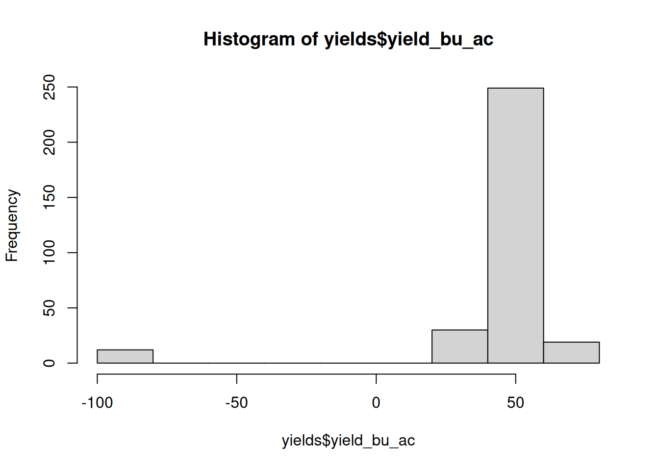
(b) The minimum is -99, which is not a yield – it is the code the office uses for a field that was never harvested. Left in, it drags the mean down.
library(tidyverse)# (a) read and summariseyields <-read_csv("data/module03/q21_yield_sentinel.csv", show_col_types =FALSE)summary(yields$yield_bu_ac)hist(yields$yield_bu_ac)# (c) -99 is a missing-value code, not a yieldclean <- yields |>mutate(yield_bu_ac =if_else(yield_bu_ac ==-99, NA, yield_bu_ac)) |>filter(!is.na(yield_bu_ac))summary(clean$yield_bu_ac)
> library(tidyverse)
>
> # (a) read and summarise
> yields <- read_csv("data/module03/q21_yield_sentinel.csv", show_col_types = FALSE)
> summary(yields$yield_bu_ac)
   Min. 1st Qu.  Median    Mean 3rd Qu.    Max.
 -99.00   43.72   48.15   42.86   52.59   68.82
> hist(yields$yield_bu_ac)
>
> # (c) -99 is a missing-value code, not a yield
> clean <- yields |>
+   mutate(yield_bu_ac = if_else(yield_bu_ac == -99, NA, yield_bu_ac)) |>
+   filter(!is.na(yield_bu_ac))
> summary(clean$yield_bu_ac)
   Min. 1st Qu.  Median    Mean 3rd Qu.    Max.
  28.50   44.31   48.42   48.57   52.74   68.82
Question 22
Tool: RThe file q22_yield_units.csv has one row per field and its spring wheat yield, in a column labelled bu/ac, for 290 fields. A bushel of wheat weighs 60 lb.
(a) [4 marks] Read the file and report the minimum, mean and maximum of yield_bu_ac, and draw a histogram of it.
(b) [3 marks] Something in this column is wrong. Say what it is, and which statistic shows it.
(c) [3 marks] Read the data into R, correcting the problem you identified in part (b), then recompute the summary on the corrected column.
Answer
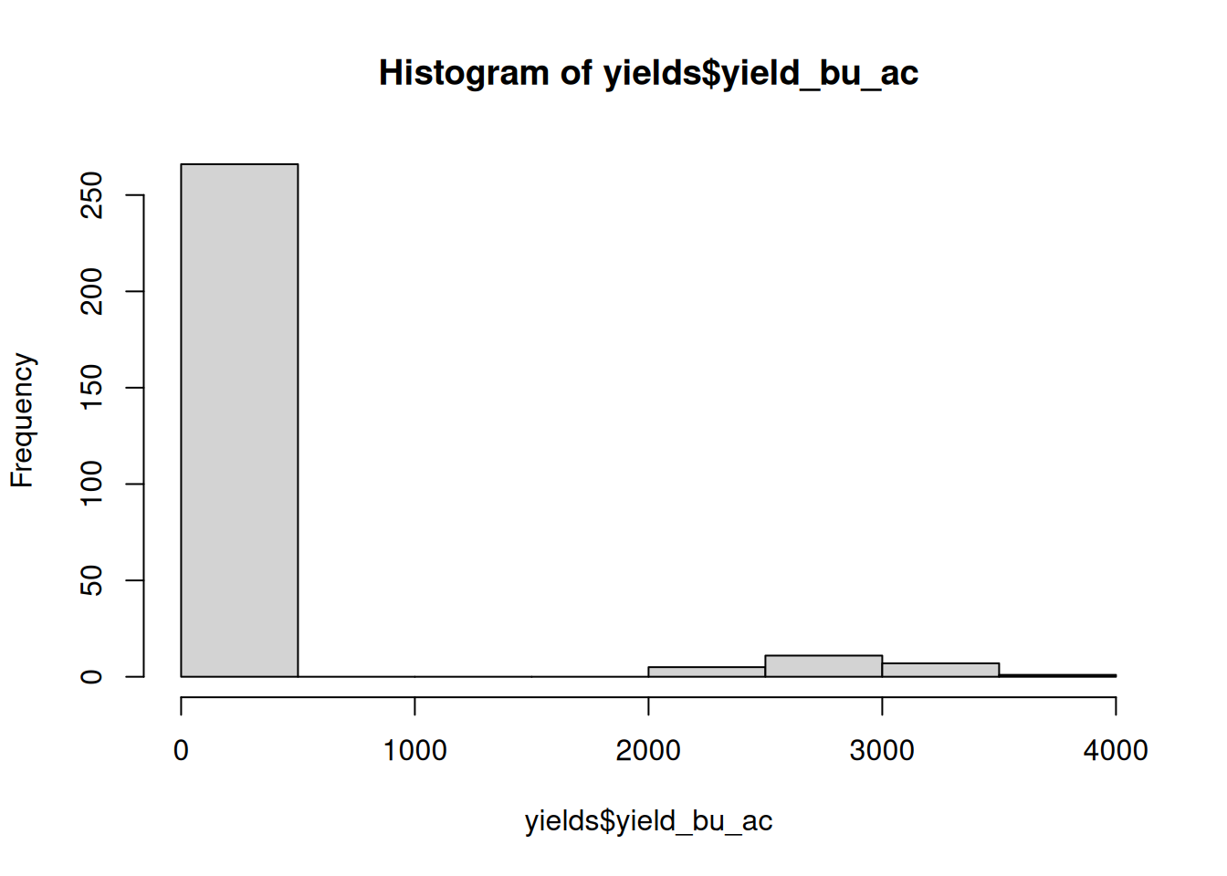
(b) The maximum is in the thousands. Some rows were recorded in lb/ac, so one column holds two units.
library(tidyverse)# (a) read and summariseyields <-read_csv("data/module03/q22_yield_units.csv", show_col_types =FALSE)summary(yields$yield_bu_ac)hist(yields$yield_bu_ac)# (c) the rows in the thousands are lb/ac; convert them to bu/acclean <- yields |>mutate(yield_bu_ac =if_else(yield_bu_ac >200, yield_bu_ac /60, yield_bu_ac))summary(clean$yield_bu_ac)
> library(tidyverse)
>
> # (a) read and summarise
> yields <- read_csv("data/module03/q22_yield_units.csv", show_col_types = FALSE)
> summary(yields$yield_bu_ac)
   Min. 1st Qu.  Median    Mean 3rd Qu.    Max.
  22.08   44.33   49.14  278.78   54.61 3631.09
> hist(yields$yield_bu_ac)
>
> # (c) the rows in the thousands are lb/ac; convert them to bu/ac
> clean <- yields |>
+   mutate(yield_bu_ac = if_else(yield_bu_ac > 200, yield_bu_ac / 60, yield_bu_ac))
> summary(clean$yield_bu_ac)
   Min. 1st Qu.  Median    Mean 3rd Qu.    Max.
  22.08   43.98   48.00   48.45   52.72   73.14
Question 23
Tool: RThe file q23_moisture_decimal.csv holds one row per delivery ticket, with the date and the moisture percentage, for 270 tickets.
(a) [4 marks] Read the file and report the minimum, mean and maximum of moisture_pct, and draw a histogram of it.
(b) [3 marks] Something in this column is wrong. Say what it is, and which statistic shows it.
(c) [3 marks] Read the data into R, correcting the problem you identified in part (b), then recompute the summary.
Answer
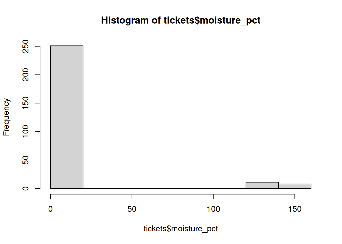
(b) The maximum is over 100, which is impossible for a percentage – the decimal point was dropped on some rows, so 13.4 became 134.
library(tidyverse)# (a) read and summarisetickets <-read_csv("data/module03/q23_moisture_decimal.csv", show_col_types =FALSE)summary(tickets$moisture_pct)hist(tickets$moisture_pct)# (c) readings over 100 lost their decimal pointclean <- tickets |>mutate(moisture_pct =if_else(moisture_pct >100, moisture_pct /10, moisture_pct))summary(clean$moisture_pct)
> library(tidyverse)
>
> # (a) read and summarise
> tickets <- read_csv("data/module03/q23_moisture_decimal.csv", show_col_types = FALSE)
> summary(tickets$moisture_pct)
   Min. 1st Qu.  Median    Mean 3rd Qu.    Max.
  10.31   12.82   13.62   22.07   14.41  151.80
> hist(tickets$moisture_pct)
>
> # (c) readings over 100 lost their decimal point
> clean <- tickets |>
+   mutate(moisture_pct = if_else(moisture_pct > 100, moisture_pct / 10, moisture_pct))
> summary(clean$moisture_pct)
   Min. 1st Qu.  Median    Mean 3rd Qu.    Max.
  10.31   12.74   13.54   13.49   14.19   16.51
Question 24
Tool: RThe file q24_field_dupes.csv holds one row per field with its acres and yield. Part of the file was pasted in a second time.
(a) [4 marks] Read the file and report the row count, the number of distinct rows, and the minimum, mean and maximum of acres. Draw a histogram of the acres.
(b) [3 marks] Identify the two problems with this data, and state which result in part (a) reveals each one.
(c) [3 marks] Read the data into R, correcting the problems you identified in part (b), then report the row count and recompute the summary.
Answer
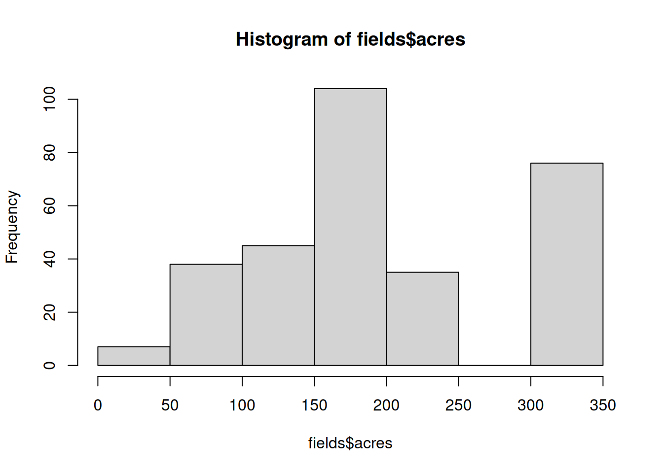
(b) Two things. The distinct-row count is lower than the row count, so some rows appear twice. And the minimum acres is 0, which no real field has.
library(tidyverse)# (a) read, count the rows and the distinct rows, and summarisefields <-read_csv("data/module03/q24_field_dupes.csv", show_col_types =FALSE)nrow(fields)nrow(distinct(fields))summary(fields$acres)hist(fields$acres)# (c) drop the repeated rows and the impossible zero-acre fieldsclean <- fields |>distinct() |>filter(acres >0)nrow(clean)summary(clean$acres)
> library(tidyverse)
>
> # (a) read, count the rows and the distinct rows, and summarise
> fields <- read_csv("data/module03/q24_field_dupes.csv", show_col_types = FALSE)
> nrow(fields)
[1] 305
> nrow(distinct(fields))
[1] 280
> summary(fields$acres)
   Min. 1st Qu.  Median    Mean 3rd Qu.    Max.
    0.0   120.0   160.0   189.5   240.0   320.0
> hist(fields$acres)
>
> # (c) drop the repeated rows and the impossible zero-acre fields
> clean <- fields |>
+   distinct() |>
+   filter(acres > 0)
> nrow(clean)
[1] 273
> summary(clean$acres)
   Min. 1st Qu.  Median    Mean 3rd Qu.    Max.
   80.0   120.0   160.0   193.4   320.0   320.0
Question 25
Tool: RThe file q25_load_weights.csv holds one row per truckload, with the elevator and the weight, which should be in kilograms, for 260 loads.
(a) [3 marks] Read the file and report the type R gives the weight_kg column. Explain why a valid minimum, mean, maximum and histogram cannot yet be calculated.
(b) [3 marks] Identify the two units used in the column and describe the text that reveals each one.
(c) [4 marks] Read the data into R, converting every weight to kilograms. Report the minimum, mean and maximum and draw a histogram of the cleaned column.
Answer
(b) The column reads in as text (<chr>), not a number, so it will not average. Some weights had the unit typed into the cell – most as kg, a few as t – so the column is text holding two different units.
library(tidyverse)# (a) the column reads in as text, so none of the statistics can be computedloads <-read_csv("data/module03/q25_load_weights.csv", show_col_types =FALSE)class(loads$weight_kg)## (b) Some weights carry a kg suffix and a few carry a t suffix, so the## column holds two units written as text.# (c) pull out the number, then scale the rows recorded in tonnesclean <- loads |>mutate(value =parse_number(weight_kg),# a load of 40 t and one of 40000 kg are the same weightweight_kg =if_else(value <1000, value *1000, value) )summary(clean$weight_kg)hist(clean$weight_kg)
> library(tidyverse)
>
> # (a) the column reads in as text, so none of the statistics can be computed
> loads <- read_csv("data/module03/q25_load_weights.csv", show_col_types = FALSE)
> class(loads$weight_kg)
[1] "character"
>
> ## (b) Some weights carry a kg suffix and a few carry a t suffix, so the
> ## column holds two units written as text.
>
> # (c) pull out the number, then scale the rows recorded in tonnes
> clean <- loads |>
+   mutate(
+     value = parse_number(weight_kg),
+     # a load of 40 t and one of 40000 kg are the same weight
+     weight_kg = if_else(value < 1000, value * 1000, value)
+   )
> summary(clean$weight_kg)
   Min. 1st Qu.  Median    Mean 3rd Qu.    Max.
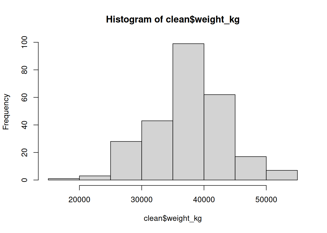
  15657   34097   38090   37627   41154   54643
> hist(clean$weight_kg)
Section 6 — Merging data in Excel
These questions are about combining tables in Power Query with Merge Queries: choosing the key, picking the join kind, and checking afterwards that you still have the rows you expect.
Question 26
Tool: Excel (Power Query)The file q26_fields.csv has one row per field, identified by field_id. The file q26_soil.csv has one row per field, identified by Field, with the soil zone and organic matter percent.
(a) [6 marks] The key has different names in the two tables. Merge them, matching field_id to Field, and report the row counts before and after.
(b) [4 marks] Compute the mean yield in each soil zone, for each crop separately. In a cell: why would a single mean yield per soil zone, across all the crops, not be worth reporting?
Tool: Excel (Power Query)Two files. q27_field_years.csv has one row per field and year with the canola yield and the field’s nearest weather station. q27_rain.csv has one row per station and year with May to August precipitation in millimetres.
(a) [6 marks] Merge the precipitation onto the yields, matching on station and year together. Report the row count before and after.
(b) [4 marks] In a cell below the table: why does this merge need two columns in its key, and what happens if you match on station alone?
Tool: Excel (Power Query)Two files. q28_fields_2024.csv is the field register for 2024 and q28_fields_2025.csv is the register for 2025. Some fields were given up between the two years and some were taken on.
(a) [5 marks] Merge the two registers on field, keeping every field that appears in either year.
(b) [5 marks] Report how many fields were farmed in both years, how many were dropped after 2024, and how many were new in 2025.
Tool: Excel (Power Query)The file q30_fields.csv has one row per field with the crop, acres and yield in bu/ac. The file q30_prices.csv has one row per crop with the price in dollars per bushel.
(a) [6 marks] Merge the price onto every field and report the row counts before and after.
(b) [4 marks] Compute each field’s revenue and the total for the farm.
The same problems in R with the dplyr joins – left_join(), inner_join(), right_join() and full_join() – including checking for keys that fail to match.
Question 31
Tool: RThe file q31_fields.csv has one row per field, with the harvest year, the crop, the acres and the yield. The file q31_prices.csv gives the price per bushel for each crop in each year.
(a) [4 marks] Join the prices onto the fields, matching on crop and year. Report the row counts before and after.
(b) [3 marks] In a comment: what happens if you join on crop alone, and why is the result wrong?
(c) [3 marks] Compute the total revenue for the farm.
Answer
# (a) The price depends on both the crop and the yearfields <-read_csv("data/module03/q31_fields.csv", show_col_types =FALSE)prices <-read_csv("data/module03/q31_prices.csv", show_col_types =FALSE)priced <- fields |>left_join(prices, by =join_by(crop, year))nrow(fields)nrow(priced)# (b) Joining on crop alone matches both price years to every fieldnrow(left_join(fields, prices, by =join_by(crop)))## (b) Twenty fields become forty rows, because each field matches its## crop in both 2024 and 2025. Half of those rows price the harvest with## the wrong year, and a revenue total over them counts every field twice.# (c) Total revenuepriced |>mutate(revenue = yield_bu_ac * acres * price_per_bu) |>summarise(total_revenue =sum(revenue))
> # (a) The price depends on both the crop and the year
> fields <- read_csv("data/module03/q31_fields.csv", show_col_types = FALSE)
> prices <- read_csv("data/module03/q31_prices.csv", show_col_types = FALSE)
> priced <- fields |>
+   left_join(prices, by = join_by(crop, year))
> nrow(fields)
[1] 20
> nrow(priced)
[1] 20
>
> # (b) Joining on crop alone matches both price years to every field
> nrow(left_join(fields, prices, by = join_by(crop)))
Warning: Detected an unexpected many-to-many relationship between `x` and `y`.
ℹ Row 1 of `x` matches multiple rows in `y`.
ℹ Row 3 of `y` matches multiple rows in `x`.
ℹ If a many-to-many relationship is expected, set `relationship =
  "many-to-many"` to silence this warning.
[1] 40
>
> ## (b) Twenty fields become forty rows, because each field matches its
> ## crop in both 2024 and 2025. Half of those rows price the harvest with
> ## the wrong year, and a revenue total over them counts every field twice.
>
> # (c) Total revenue
> priced |>
+   mutate(revenue = yield_bu_ac * acres * price_per_bu) |>
+   summarise(total_revenue = sum(revenue))
# A tibble: 1 × 1
  total_revenue
          <dbl>
1      1796242.
Question 32
Tool: RNo data file for this question. Two tables, A and B, are joined on a single key column. A has 30 rows and B has 40. Every row of A finds a match in B, and each one matches a different B row, so 30 of B’s rows are matched and the other 10 are not.
(a) [7 marks] In comments in your script, give the number of rows returned by each of these, and say in one line why:
left_join(A, B)
full_join(A, B)
right_join(A, B)
(b) [3 marks] In a comment: which of the three would you use to build a table of B’s rows and nothing else, whether or not each one was matched?
Answer
# (a)# left_join(A, B) -> 30 rows. A left join keeps every row of A, and each# of the 30 finds exactly one match, so nothing is added or dropped.## full_join(A, B) -> 40 rows. Every row of A is kept (30), plus the rows# of B that never matched. B has 40 rows and 30 of them match, so 10 are# unmatched: 30 + 10 = 40.## right_join(A, B) -> 40 rows. A right join keeps every row of B. The 30# matched rows pick up their A columns and the 10 unmatched ones get NA.# (b) The right join. The full join gives the same 40 rows here, but only# because every row of A happens to match; the right join is the one that# keeps B's rows whatever A contains.
Question 33
Tool: RThe file q28_fields_2024.csv lists the fields farmed in 2024 with that year’s crop; q28_fields_2025.csv does the same for 2025. Some fields were rented out after 2024 and some were taken on in 2025.
(a) [4 marks] Use full_join() to build one table with every field from either year, and report its row count.
(b) [4 marks] From that table, report how many fields were farmed in both years, how many were dropped after 2024, and how many were new in 2025. A field that was in only one year has NA in the other year’s columns, so is.na() will find it.
(c) [2 marks] In a comment: why do both files’ acres columns end up in the result, and what are they called?
Answer
# (a) Every field from either yearf24 <-read_csv("data/module03/q28_fields_2024.csv", show_col_types =FALSE)f25 <-read_csv("data/module03/q28_fields_2025.csv", show_col_types =FALSE)both <-full_join(f24, f25, by =join_by(field))nrow(both)# (b) A missing crop marks a year the field was not farmedboth |>summarise(in_both =sum(!is.na(crop_2024) &!is.na(crop_2025)),dropped =sum(!is.na(crop_2024) &is.na(crop_2025)),new_in_25 =sum( is.na(crop_2024) &!is.na(crop_2025)) )## (c) Both files have an acres column and it is not part of the key, so## the join keeps both and adds a suffix to tell them apart: acres.x from## the 2024 table and acres.y from the 2025 table.
> # (a) Every field from either year
> f24 <- read_csv("data/module03/q28_fields_2024.csv", show_col_types = FALSE)
> f25 <- read_csv("data/module03/q28_fields_2025.csv", show_col_types = FALSE)
> both <- full_join(f24, f25, by = join_by(field))
> nrow(both)
[1] 20
>
> # (b) A missing crop marks a year the field was not farmed
> both |>
+   summarise(
+     in_both   = sum(!is.na(crop_2024) & !is.na(crop_2025)),
+     dropped   = sum(!is.na(crop_2024) &  is.na(crop_2025)),
+     new_in_25 = sum( is.na(crop_2024) & !is.na(crop_2025))
+   )
# A tibble: 1 × 3
  in_both dropped new_in_25
    <int>   <int>     <int>
1      13       3         4
>
> ## (c) Both files have an acres column and it is not part of the key, so
> ## the join keeps both and adds a suffix to tell them apart: acres.x from
> ## the 2024 table and acres.y from the 2025 table.
Question 34
Tool: RThe file q34_deliveries.csv has one row per delivery ticket with the field name and the weight. The file q34_fields.csv is the field register. Three tickets have the field name mistyped.
(a) [4 marks] Left join the register onto the deliveries and filter to the rows where the crop came back NA. Those are the tickets whose field name is not in the register.
(b) [3 marks] In a comment: for each, which field was meant, and how can you tell? Then fix them with if_else().
(c) [3 marks] Join again and compute total tonnes by crop. In a comment: what would the crop totals have looked like if you had not fixed the names?
Answer
# (a) A left join keeps every ticket; an unmatched one has no cropdeliveries <-read_csv("data/module03/q34_deliveries.csv",col_types =cols(ticket_id =col_character()))fields <-read_csv("data/module03/q34_fields.csv", show_col_types =FALSE)deliveries |>left_join(fields, by =join_by(field)) |>filter(is.na(crop))## (b) Kestral is Kestrel, Meadow Vale is Meadowvale, home is Home: each## is one letter, a space or a capital away from a name in the register.# (b) Fix the three namesdeliveries <- deliveries |>mutate(field =if_else(field =="Kestral", "Kestrel", field),field =if_else(field =="Meadow Vale", "Meadowvale", field),field =if_else(field =="home", "Home", field))# (c) Tonnes by crop, now that every ticket matchesdeliveries |>left_join(fields, by =join_by(field)) |>group_by(crop) |>summarise(tonnes =sum(weight_tonnes))## (c) The three tickets would have NA for crop, so an extra group named## NA would hold their 96.7 tonnes. Barley would be short one ticket## (119.7 rather than 152.0) and Spring Wheat short two (183.2 rather## than 247.6). The other crops are unaffected.
> # (a) A left join keeps every ticket; an unmatched one has no crop
> deliveries <- read_csv("data/module03/q34_deliveries.csv",
+                        col_types = cols(ticket_id = col_character()))
> fields <- read_csv("data/module03/q34_fields.csv", show_col_types = FALSE)
> deliveries |>
+   left_join(fields, by = join_by(field)) |>
+   filter(is.na(crop))
# A tibble: 3 × 6
  ticket_id field       weight_tonnes crop  acres yield_bu_ac
  <chr>     <chr>               <dbl> <chr> <dbl>       <dbl>
1 05710     Meadow Vale          32.3 <NA>     NA          NA
2 05723     home                 24.6 <NA>     NA          NA
3 05728     Kestral              39.8 <NA>     NA          NA
>
> ## (b) Kestral is Kestrel, Meadow Vale is Meadowvale, home is Home: each
> ## is one letter, a space or a capital away from a name in the register.
>
> # (b) Fix the three names
> deliveries <- deliveries |>
+   mutate(field = if_else(field == "Kestral", "Kestrel", field),
+          field = if_else(field == "Meadow Vale", "Meadowvale", field),
+          field = if_else(field == "home", "Home", field))
>
> # (c) Tonnes by crop, now that every ticket matches
> deliveries |>
+   left_join(fields, by = join_by(field)) |>
+   group_by(crop) |>
+   summarise(tonnes = sum(weight_tonnes))
# A tibble: 5 × 2
  crop         tonnes
  <chr>         <dbl>
1 Barley         152
2 Canola         168.
3 Oats           144.
4 Peas           187.
5 Spring Wheat   248.
>
> ## (c) The three tickets would have NA for crop, so an extra group named
> ## NA would hold their 96.7 tonnes. Barley would be short one ticket
> ## (119.7 rather than 152.0) and Spring Wheat short two (183.2 rather
> ## than 247.6). The other crops are unaffected.
Question 35
Tool: RThe file q35_fields.csv has one row per field with the crop, acres, yield and the unit the yield is recorded in: bu/ac for most crops, lb/ac for lentils. The file q35_units.csv has one row per crop with the factor that converts its unit to kg/ha.
(a) [4 marks] Join the conversion factors onto the fields and report the row counts.
(b) [3 marks] Compute every yield in kg/ha.
(c) [3 marks] Compute the mean yield of each crop in kg/ha, and in a comment say why the mean of the original yield column across all fields is meaningless.
Answer
# (a) Conversion factors onto fieldsfields <-read_csv("data/module03/q35_fields.csv")units <-read_csv("data/module03/q35_units.csv")merged <- fields |>left_join(units, by =join_by(crop))nrow(fields)nrow(merged)# (b) A common unitmerged <- merged |>mutate(yield_kg_ha = yield * kg_ha_per_unit)# (c) Mean by crop in kg/hamerged |>group_by(crop) |>summarise(mean_kg_ha =mean(yield_kg_ha))## (c) The original column mixes bushels and pounds. Averaging a lentil## field at 1554.9 lb/ac with a canola field at 49.5 bu/ac adds two## different units.
> # (a) Conversion factors onto fields
> fields <- read_csv("data/module03/q35_fields.csv")
Rows: 20 Columns: 5
── Column specification ────────────────────────────────────────────────────────
Delimiter: ","
chr (3): field, crop, unit
dbl (2): acres, yield

ℹ Use `spec()` to retrieve the full column specification for this data.
ℹ Specify the column types or set `show_col_types = FALSE` to quiet this message.
> units <- read_csv("data/module03/q35_units.csv")
Rows: 5 Columns: 2
── Column specification ────────────────────────────────────────────────────────
Delimiter: ","
chr (1): crop
dbl (1): kg_ha_per_unit

ℹ Use `spec()` to retrieve the full column specification for this data.
ℹ Specify the column types or set `show_col_types = FALSE` to quiet this message.
> merged <- fields |>
+   left_join(units, by = join_by(crop))
> nrow(fields)
[1] 20
> nrow(merged)
[1] 20
>
> # (b) A common unit
> merged <- merged |>
+   mutate(yield_kg_ha = yield * kg_ha_per_unit)
>
> # (c) Mean by crop in kg/ha
> merged |>
+   group_by(crop) |>
+   summarise(mean_kg_ha = mean(yield_kg_ha))
# A tibble: 5 × 2
  crop         mean_kg_ha
  <chr>             <dbl>
1 Barley            3995.
2 Canola            2184
3 Lentils           1741.
4 Oats              3561.
5 Spring Wheat      3349.
>
> ## (c) The original column mixes bushels and pounds. Averaging a lentil
> ## field at 1554.9 lb/ac with a canola field at 49.5 bu/ac adds two
> ## different units.