This bank holds 30 questions: ten in each section.
Section 1 (Questions 1–10) covers the ideas behind spatial data: what it is, how it is stored, and how to reason about it. No code, and no file needed.
Section 2 (Questions 11–20) covers reading and mapping spatial data in R.
Saskatchewan RM boundaries. 296 rural municipalities, with rmno (the RM number) and rmnm (its name). Vector polygons in WGS 84.
SCIC grain risk zones. The 23 zones Saskatchewan Crop Insurance uses to set rates, with risk_zone. Vector polygons.
Quarter sections. The 6,390 legal quarter sections inside those four RMs, each about 160 acres, with its legal land description (lld, for example NE-16-048-05-W3) and the RM it falls in. This is the grid Saskatchewan land is bought, sold and insured on.
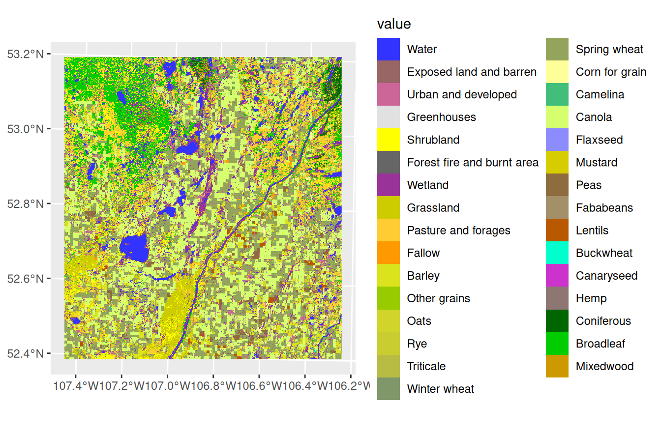
Annual Crop Inventory 2023 slice. A raster of 30-metre cells covering four RMs north-west of Saskatoon: Blaine Lake, Laird, Redberry and Leask. Each cell holds a class code.
Crop class names. What each class code means, and the colour Agriculture Canada uses for it.
Your module test will contain one question per section, and you have 50 minutes for all three. The test runs in two parts: the first in Respondus LockDown Browser with no AI, where you answer your Section 1 question and write pseudocode for the other two; the second your R script, where AI is allowed.
Where a question below names an RM, a risk zone or a crop, your test will name a different one. Everybody gets their own, so the numbers in your answer will usually be yours alone. What does not change is the steps, which is why the pseudocode is the thing to get right.
For each question, 20% of the mark is for presentation and the other 80% is for the correctness of your pseudocode, script and answers.
NoteHow the two parts work
Part 1 – in Respondus LockDown Browser, no AI. You answer your Section 1 question, and you write pseudocode for your Section 2 and Section 3 questions. LockDown Browser stops you opening anything else while you do it, so this part is from your own head. The pseudocode is marked on whether the steps are right and in the right order, not on R syntax. Chapter 18 describes the level of detail to aim for.
Part 1 is designed to take about 20 minutes, which leaves 30 for the rest. You can spend the time differently if you want to.
Part 2 – your R script, AI allowed. When you submit Part 1 the lockdown ends and Part 2 opens. Now you write and run the R that does what your pseudocode described, and you may use any AI tool you like. You upload one .R script with a header block, a labelled section for each question, and your sentence answers written as comments. It should run top to bottom in a fresh session.
Part 1 asks whether you know what the code has to do, and Part 2 asks whether you can get a working answer out of a machine that will write the syntax for you.
Section 1 — Spatial data
These questions are about what spatial data is and how it is stored. They are answered in the Canvas text box, in sentences. There is no code in this section, and you do not need any file in front of you.
Question 1
(a) What makes a dataset spatial, as opposed to an ordinary table of numbers?
(b) A vector file is described as a table with an extra column. What is in that column, and how is it unlike every other column in the table?
(c) Give an example of an agricultural question you could only answer if the location were attached to the numbers.
Answer
(a) It keeps the where attached to the numbers, so location can be part of the analysis rather than just a label. A yield belongs to a field, a rainfall reading to a gauge, an insurance rate to a risk zone.
(b) The geometry column, which holds the shape of the thing in that row – a list of coordinate pairs that trace it. Every other column holds one value per row: a number, a name. The geometry column holds a whole shape in each entry.
(c) Any question that depends on where things are rather than only what they are: which RMs border the one a producer farms in, which risk zone a field falls in, whether the low-yielding RMs are next to each other or scattered across the province. Without the location you have the yields but no way to ask any of those.
Question 2
(a) What does the geometry of a polygon represent, and why does its last point repeat its first?
(b) A polygon has these five points, in this order:
Point
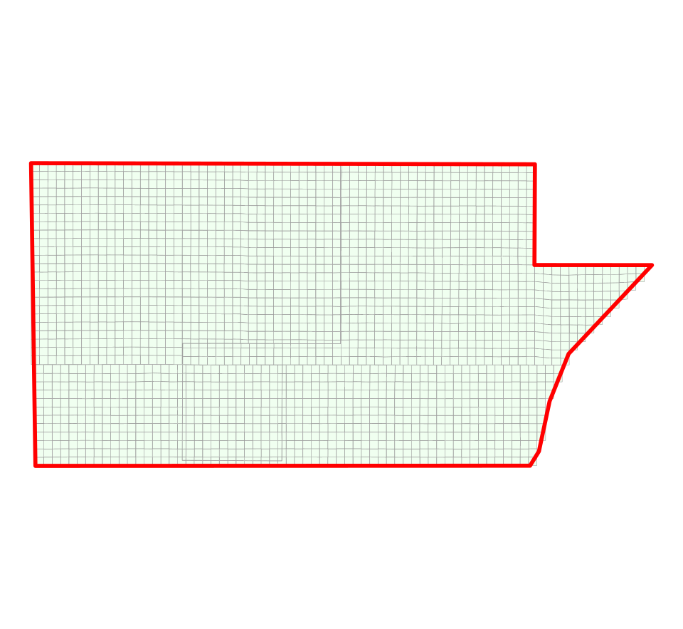
x
y
1
0
0
2
4
0
3
4
3
4
0
3
5
0
0
Describe the shape, and give its area.
(c) A sixth point, (2, 5), is added to the list immediately before the closing point, so the order becomes (0,0), (4,0), (4,3), (0,3), (2,5), (0,0). Describe what this traces, and say whether it is a valid polygon.
Answer
(a) It is a list of points, each a coordinate pair. Connect them in the order they are stored and you trace the boundary of the shape. The last point repeats the first so the boundary closes – without it you have a line that stops short rather than an enclosed area.
(b) A rectangle 4 wide and 3 tall, so the area is 12.
(c) It is not a valid polygon. The boundary runs along the top to (0,3), up to the peak at (2,5), and then straight back down to (0,0) – and that last edge cuts across the top edge on its way. The two edges cross at (1.2, 3), so there is no single inside and no area to measure.
Putting the new point between (4,3) and (0,3) instead would give the house shape it was meant to be, with an area of 16. The points are the same either way; where one sits in the list decides whether the shape is valid.
Question 3
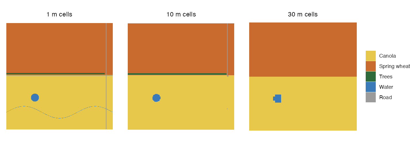
The same square of farmland, recorded three times at three different cell sizes. The legend names every land type the classifier can assign.
(a) Three of the land types in the first panel have gone by the last one. Name them, and explain why they disappeared.
(b) They do not all disappear at the same step. Put them in order of how wide they are on the ground, and say how the panels told you.
(c) The slough survives all three panels but looks different in the last one. What has happened to it?
(d) You are asked how much of this land is canola, and separately where a culvert would be needed. Which panel would you use for each?
Answer
(a) The creek, the roads and the shelterbelt. Each is narrower than a 30-metre cell. A cell holds one value for all the ground it covers and takes whichever class covers most of it, so none of these is ever the majority of a cell at that size, and every cell they run through is recorded as the crop around them instead. They are not hidden in the coarse panel – they are absent from it.
(b) Creek narrowest, then the roads, then the shelterbelt. The creek and the roads are both gone by the middle panel, so both are under 10 metres; the shelterbelt survives it and is lost only at 30, so it is between 10 and 30 metres wide. Within the first two, the creek is drawn as a thinner line than the roads in the 1-metre panel. The panels let you bracket each feature’s width without being told it.
(c) It survives because it is far wider than any of the cells, so it is the majority of many cells rather than a minority of a few. What changes is its edge: a boundary can only follow cell edges, so the round shape becomes blocky, and at 30 metres it is a rough square. The feature is still there and its shape is now approximate.
(d) For the canola acreage, the 30-metre panel is fine. The features it lost are a small share of the area, so the acreage is off by a little, and far less than the error in the classification itself. For siting a culvert you need the 1-metre panel, because a culvert goes where the creek crosses the road and neither the creek nor the road exists in the other two. No care in the analysis recovers them.
Question 4
(a) Why does putting the earth’s surface on a flat map distort it?
(b) Why is there no single agreed coordinate reference system that everyone uses for flat maps?
(c) Two layers you want to use together are in different coordinate reference systems. What has to happen before you can combine them?
Answer
(a) The earth is curved and a map is flat. A curved surface cannot be laid out flat without being stretched or torn, so something has to give: shapes, areas, distances or directions come out wrong somewhere on the map.
(b) Because there is no projection that gets everything right. Flattening the earth always distorts shape, area, distance or direction, and a projection can only preserve some of those at the cost of the others. Which trade is the right one depends on what the map is for and what part of the world it covers, so different purposes settle on different systems and no single one is best for all of them.
(c) One of them has to be converted so that both are in the same system. Until then the two sets of coordinates are measured in different units from different origins, so the same ground has different numbers in each layer and nothing can be compared between them.
Question 5
(a) A location is usually written as a longitude and a latitude, but the order they go in varies. What is the order in R, and why?
(b) A point in Saskatchewan is entered the wrong way round. Why does that mistake announce itself, and where in the world would it not?
(c) You build a table of Saskatchewan locations from a GPS unit, which lists latitude first, and turn it into spatial data without reordering the columns. What will the map look like?
Answer
(a) Longitude first, because longitude is the x coordinate and latitude is the y. Maps, GPS units and Google write latitude first, which is where the confusion comes from.
(b) Swapped, the latitude becomes about -106, and latitude only runs from -90 to 90. It is not a possible location, so the error shows up straight away. Every Saskatchewan longitude is beyond -90, so the swap always fails here. Nearer the equator both numbers are small enough to be valid either way round, and the swap puts you somewhere real and wrong, which is much harder to notice.
(c) R raises no error. It takes the first column as longitude and the second as latitude, stores the pair exactly as given, and draws it. Every point ends up at about 52 degrees east and 106 degrees south – off the bottom of the world, far from Saskatchewan – so the map stretches to cover both the points and the province, and the RMs shrink to a speck in one corner. The mistake shows up in the picture, not in a message.
Question 6
(a) Define resolution and extent.
(b) A raster has 30-metre cells, 1,500 rows and 2,000 columns. What is its resolution, and what is its extent?
Answer
(a) Resolution is the size of the smallest thing the data can tell apart – for a raster, the cell. Extent is how much ground the data covers.
(b) The resolution is 30 metres – the cell size. The extent is the ground it covers: 2,000 columns at 30 metres is 60 km across, and 1,500 rows at 30 metres is 45 km down, so 60 km by 45 km. That is 3 million cells covering 2,700 square kilometres.
Question 7
(a) Explain the difference between a raster whose values are continuous and one whose values are categorical.
(b) In a land cover raster, 146 is spring wheat and 153 is canola. Why is the average of those two values meaningless?
(c) How should values be mapped differently depending on whether they are continuous or categorical?
Answer
(a) Continuous values have a natural numbering on some scale or unit, so arithmetic on them means something: yield in bushels per acre, rainfall in millimetres. Categorical values have no natural numbering – the number is only a code for a class, like 153 for canola, and could have been any other number.
(b) The numbers are codes, not quantities. Their average is 149.5, which is not half-way between two crops – it is either another crop’s code or no class at all. Codes that are close together are not any more similar than codes that are far apart, so the gap of 7 between them measures nothing.
(c) Continuous values can be drawn with a colour gradient, where darker shades usually mean higher values, because the reader is meant to see the order and read a value off the scale. Categorical values need a separate colour for each class, chosen so the classes are easy to tell apart. Putting a gradient on categories gives near-identical shades to codes that happen to be close together, and invites the reader to see an order that is not there.
Question 8
A quarter section is about 800 metres on a side, and is mostly planted to canola. But it also contains two narrow creeks that are a bit over 1 m wide and 100 m long, and a shelterbelt of trees about 15 m wide running the full 800 m length of the quarter.
(a) If you mapped this land with a raster at a resolution of 10 metres, approximately how many cells do you think would be categorized as canola, water, and trees?
(b) How would this change if you used a raster with a resolution of 1 metre instead?
(c) If your goal was measuring total land devoted to canola – do you think the different resolutions would matter? What if your goal was mapping out water flow in Saskatchewan?
Answer
(a) At 10 metres the quarter is 80 cells by 80, so 6,400 cells in total.
The creeks are a tenth of a cell wide, so no cell is mostly water and none is classed as water. They disappear. The shelterbelt is 15 metres wide, so it covers one and a half cells across and runs the 80 cells down the quarter – it survives as a strip one or two cells wide, somewhere around 80 to 160 cells of trees. Everything else, roughly 6,250 cells, comes back as canola.
(b) At 1 metre the quarter is 800 by 800, so 640,000 cells.
Now both features are wider than a cell. The creeks come out at about 200 cells of water and the shelterbelt at about 12,000 cells of trees, both close to the ground they really cover. The canola is about 628,000 cells.
(c) For total canola it hardly matters. The creeks are 200 square metres out of 640,000, and even losing the shelterbelt entirely would move the canola figure by under 2%, which is smaller than the error in the classification itself. For mapping water flow the coarse raster is useless: the creeks are exactly what you are trying to map and the 10-metre raster does not contain them at all. No amount of careful work on that file recovers them, because the information was gone before you opened it.
Question 9
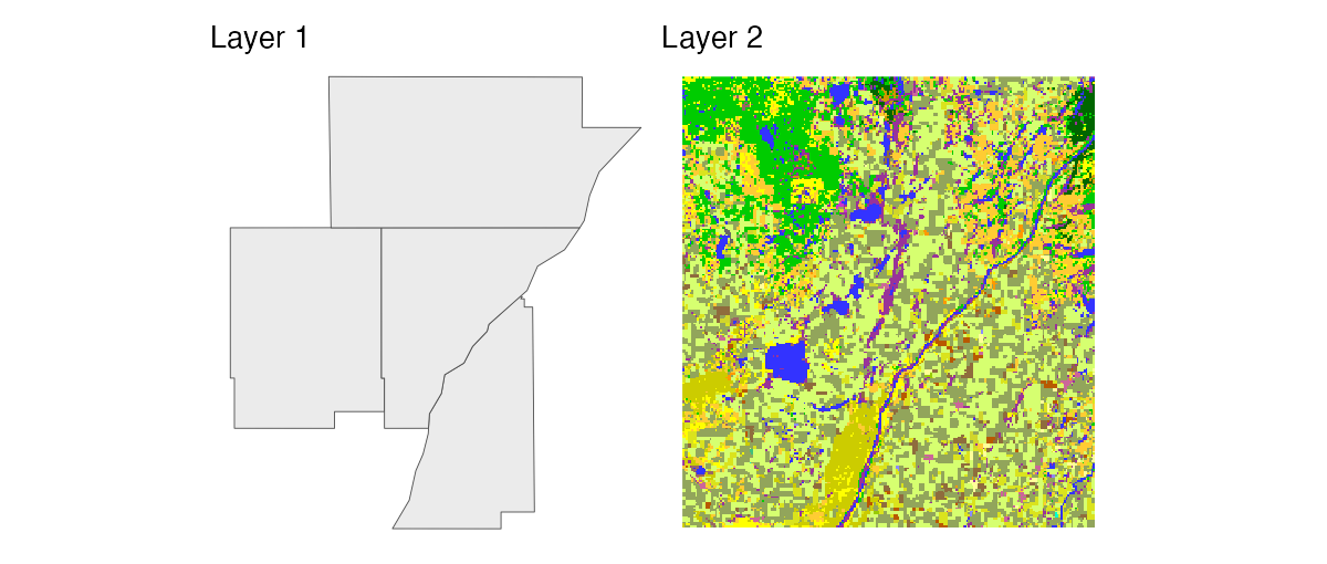
The two pictures below show the same part of Saskatchewan, from two different files.
(a) Which layer is vector and which is raster? How can you tell by looking?
(b) Layer 1 has four shapes in it. How many rows would you expect in its table, and what would the geometry column of one row hold?
(c) Layer 2 covers less ground than Layer 1 but is a much larger file. Explain why.
Answer
(a) Layer 1 is vector and Layer 2 is raster. Layer 1 is a handful of outlined shapes whose edges run where the real boundaries run, including the irregular ones. Layer 2 is a grid of small squares of equal size, and every edge in it follows cell edges, which is why the river has a stepped look.
(b) Four rows, one per shape. The geometry column of one row would hold the list of coordinate pairs tracing that shape’s boundary, closing back on its first point.
(c) Layer 1 stores only the corner points of four boundaries, which is a few hundred numbers. Layer 2 stores a value for every cell across its whole extent whether anything is happening there or not, and at 30 metres that is millions of values.
Question 10
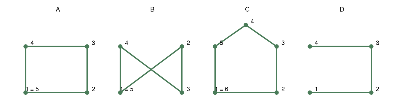
Each picture below is one polygon. The dots are the points as they are stored, numbered in storage order, and the line joins them in that order.
(a) Which of these four is a valid polygon with an area you could measure? Explain what is wrong with each of the others.
(b) A and B are built from exactly the same four corner points. Why do they look different?
(c) What single change would turn D into a valid polygon?
Answer
(a) A and C are valid: both close back on their first point and neither crosses itself, so each encloses an area. B crosses itself, so there is no single inside – the two triangles are on opposite sides of the crossing and the shape has no well-defined area. D never returns to its first point, so it is an open line rather than an enclosed shape.
(b) The points are the same but the order is not. A joins them around the outside; B goes corner to opposite corner and back, so two of the edges cross in the middle. The order the points are stored in is part of the geometry, not just a way of listing the corners.
(c) Add a fifth point repeating the first, so the boundary closes.
Section 2 — Reading and mapping
For each of these you write pseudocode in Part 1 and an R script in Part 2. The pseudocode should name the file you are reading and say what each step does, without worrying about function names. Your test will name a different RM, zone or crop from the one below.
Question 11
This question uses sask_rms.geojson.
(a) Read the RM boundaries and report how many rows and columns the file has.
(b) Report the coordinate reference system it arrived in.
(c) Make a map of all 296 RMs, with the RM of Blaine Lake filled in dark green and the rest left grey.
Answer
Pseudocode
read sask_rms.geojson         (one row per rural municipality)
  report how many rows and columns it has
  report the coordinate reference system

pull out the one row where the RM name is BLAINE LAKE

map all the RMs in grey
  draw the Blaine Lake row on top of them in dark green
R code
rms <-st_read("data/sask_rms.geojson", quiet =TRUE) |>clean_names()##(a) rows and columnsdim(rms)##(b) the CRS it arrived inst_crs(rms)$Name##(c) the one RM we wantblaine <-filter(rms, rmnm =="BLAINE LAKE")
> rms <- st_read("data/sask_rms.geojson", quiet = TRUE) |>
+   clean_names()
>
> ##(a) rows and columns
> dim(rms)
[1] 296   3
>
> ##(b) the CRS it arrived in
> st_crs(rms)$Name
[1] "WGS 84"
>
> ##(c) the one RM we want
> blaine <- filter(rms, rmnm == "BLAINE LAKE")
ggplot() +geom_sf(data = rms, fill ="grey95", colour ="grey70") +geom_sf(data = blaine, fill ="darkgreen") +theme_void()
Question 12
This question uses sask_rms.geojson and rm_yields_1990_2025.csv.
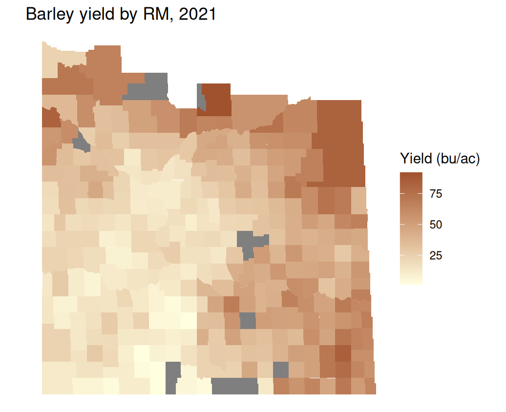
(a) Read both files and join the 2021 barley yields onto the RM boundaries.
(b) Report how many RMs have no 2021 barley yield.
(c) Map the result, with yield shown by fill colour. Give the map a title and a legend label.
Answer
Pseudocode
read sask_rms.geojson           (one row per RM)
read rm_yields_1990_2025.csv    (one row per RM, year and crop)

keep only the rows where the year is 2021 and the crop is barley
join those yields onto the boundaries, matching RM number to RM number

count how many RMs ended up with no yield

map the RMs with the fill colour set by yield
  title it, and label the legend
R code
rms <-st_read("data/sask_rms.geojson", quiet =TRUE) |>clean_names() |>mutate(rmno =as.numeric(rmno))yields <-read_csv("data/rm_yields_1990_2025.csv", show_col_types =FALSE) |>clean_names()##(a) the 2021 barley yields, joined onbarley <-filter(yields, year ==2021, crop =="Barley")rms_barley <-left_join(rms, barley, by =c("rmno"="rm"))##(b) RMs with no yield recordedsum(is.na(rms_barley$yield))
> rms <- st_read("data/sask_rms.geojson", quiet = TRUE) |>
+   clean_names() |>
+   mutate(rmno = as.numeric(rmno))
>
> yields <- read_csv("data/rm_yields_1990_2025.csv", show_col_types = FALSE) |>
+   clean_names()
>
> ##(a) the 2021 barley yields, joined on
> barley <- filter(yields, year == 2021, crop == "Barley")
> rms_barley <- left_join(rms, barley, by = c("rmno" = "rm"))
>
> ##(b) RMs with no yield recorded
> sum(is.na(rms_barley$yield))
[1] 10
This question uses aci_slice_2023.tif and aci_crop_classes.csv.
(a) Read the raster and report its dimensions and cell size.
(b) Print a 10-by-10 block of its values, taken from rows 1380 to 1389 and columns 2106 to 2115.
(c) Explain in a comment what the numbers in that block represent.
Answer
Pseudocode
read aci_slice_2023.tif      (a grid of 30 m cells)
  report how many rows and columns it has
  report the size of one cell

turn the raster into a matrix of numbers
  print rows 1380 to 1389 and columns 2106 to 2115

in a comment, say what the numbers mean
R code
aci <-rast("data/aci_slice_2023.tif")##(a) rows, columns and cell sizedim(aci)res(aci)##(b) a block of the raw valuesaci_matrix <-as.matrix(aci, wide =TRUE)aci_matrix[1380:1389, 2106:2115]##(c) Each number is a crop class code for one 30 m cell: 146 is spring##wheat, 153 is canola, 34 is urban and developed. The codes are labels,##not quantities.
> aci <- rast("data/aci_slice_2023.tif")
>
> ##(a) rows, columns and cell size
> dim(aci)
[1] 2997 2745    1
> res(aci)
[1] 30.02163 30.02163
>
> ##(b) a block of the raw values
> aci_matrix <- as.matrix(aci, wide = TRUE)
> aci_matrix[1380:1389, 2106:2115]
      [,1] [,2] [,3] [,4] [,5] [,6] [,7] [,8] [,9] [,10]
 [1,]  146  146  146  146   34  153  153  153  153   153
 [2,]  146  146  146  146   34  153  153  153  153   153
 [3,]  146  146  146  146   34  153  153  153  153   153
 [4,]  146  146  146  146   34  153  153  153  153   153
 [5,]  146  146  146  146   34  153  153  153  153   153
 [6,]  146  146  146  146   34  153  153  153  153   153
 [7,]  146  146  146  146   34  153  153  153  153   153
 [8,]  146  146  146  146   34  153  153  153  153   153
 [9,]  146  146  146  146   34  153  153  153  153   153
[10,]  146  146  146  146   34  153  153  153  153   153
>
> ##(c) Each number is a crop class code for one 30 m cell: 146 is spring
> ##wheat, 153 is canola, 34 is urban and developed. The codes are labels,
> ##not quantities.
Question 14
This question uses aci_slice_2023.tif and aci_crop_classes.csv.
(a) Read the raster and the class table, and attach the class names to the raster so it is categorical.
(b) Map the raster using Agriculture Canada’s own colours from the class table.
(c) In a comment: name one thing that is hard to read on this map and say why.
Answer
Pseudocode
read aci_slice_2023.tif       (a grid of crop class codes)
read aci_crop_classes.csv     (what each code means, and its colour)

attach the class table to the raster so each code carries a crop name

map the raster
  use the colour column from the class table for the fill colours

in a comment, say what is hard to read and why
R code
aci <-rast("data/aci_slice_2023.tif")classes <-read_csv("data/aci_crop_classes.csv", show_col_types =FALSE)##(a) attaching the table makes the raster categoricallevels(aci) <- classes
> aci <- rast("data/aci_slice_2023.tif")
> classes <- read_csv("data/aci_crop_classes.csv", show_col_types = FALSE)
>
> ##(a) attaching the table makes the raster categorical
> levels(aci) <- classes
(c) Canola and spring wheat are both yellow-green, so the two biggest classes are the hardest pair to tell apart. The legend runs to 31 entries, most of them classes that cover too few cells to find on the map.
Question 15
This question uses sask_rms.geojson and sk_risk_zones.geojson.
(a) Read both layers and report whether they share a coordinate reference system.
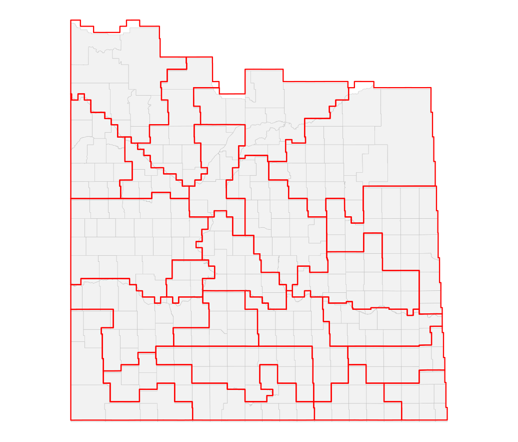
(b) Map the RM boundaries in grey with the risk zone boundaries drawn over them in red.
(c) In a comment: what does the map show about how the two layers line up?
Answer
Pseudocode
read sask_rms.geojson        (296 municipalities)
read sk_risk_zones.geojson   (23 risk zones)

check whether the two layers have the same CRS

map the RMs in grey
  draw the risk zone boundaries on top in red, with no fill

in a comment, say how the two sets of boundaries relate
R code
rms <-st_read("data/sask_rms.geojson", quiet =TRUE) |>clean_names()zones <-st_read("data/sk_risk_zones.geojson", quiet =TRUE)##(a) do they agree?st_crs(rms) ==st_crs(zones)
> rms <- st_read("data/sask_rms.geojson", quiet = TRUE) |> clean_names()
> zones <- st_read("data/sk_risk_zones.geojson", quiet = TRUE)
>
> ##(a) do they agree?
> st_crs(rms) == st_crs(zones)
[1] TRUE
ggplot() +geom_sf(data = rms, fill ="grey95", colour ="grey75", linewidth =0.1) +geom_sf(data = zones, fill =NA, colour ="red", linewidth =0.4) +theme_void()
(c) The zone boundaries cut through RMs rather than following them. A zone is not a group of whole RMs.
Question 16
This question uses sask_rms.geojson and rm_yields_1990_2025.csv.
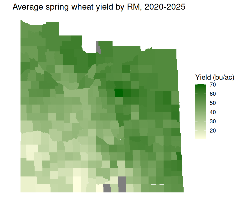
(a) Build a table of the average spring wheat yield in each RM over 2020 to 2025.
(b) Join it to the boundaries and map it.
Answer
Pseudocode
read sask_rms.geojson
read rm_yields_1990_2025.csv

keep the rows where the crop is spring wheat and the year is 2020 or later
for each RM, work out the average yield over those years

join the averages onto the boundaries

map the RMs with fill set by the average yield
  title it and label the legend
R code
rms <-st_read("data/sask_rms.geojson", quiet =TRUE) |>clean_names() |>mutate(rmno =as.numeric(rmno))yields <-read_csv("data/rm_yields_1990_2025.csv", show_col_types =FALSE) |>clean_names()##(a) the average over 2020-2025avg <- yields |>filter(crop =="Spring Wheat", year >=2020, year <=2025) |>summarise(mean_yield =mean(yield, na.rm =TRUE), .by = rm)##(b) attach it to the boundariesrms_wheat <-left_join(rms, avg, by =c("rmno"="rm"))
> rms <- st_read("data/sask_rms.geojson", quiet = TRUE) |>
+   clean_names() |>
+   mutate(rmno = as.numeric(rmno))
>
> yields <- read_csv("data/rm_yields_1990_2025.csv", show_col_types = FALSE) |>
+   clean_names()
>
> ##(a) the average over 2020-2025
> avg <- yields |>
+   filter(crop == "Spring Wheat", year >= 2020, year <= 2025) |>
+   summarise(mean_yield = mean(yield, na.rm = TRUE), .by = rm)
>
> ##(b) attach it to the boundaries
> rms_wheat <- left_join(rms, avg, by = c("rmno" = "rm"))
ggplot() +geom_sf(data = rms_wheat, aes(fill = mean_yield), colour =NA) +scale_fill_gradient(low ="lightyellow", high ="darkgreen",name ="Yield (bu/ac)") +labs(title ="Average spring wheat yield by RM, 2020-2025") +theme_void()
Question 17
This question uses sask_rms.geojson and rm_yields_1990_2025.csv.
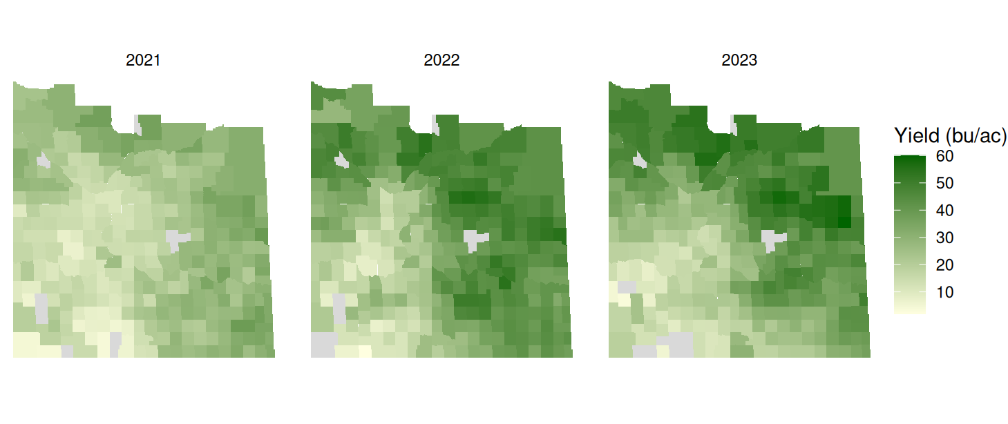
(a) Map the canola yield by RM for 2021, 2022 and 2023 as three maps side by side.
(b) Use the same fill scale across all three.
(c) In a comment: why does using one scale for all three matter?
Answer
Pseudocode
read sask_rms.geojson
read rm_yields_1990_2025.csv

for each year separately, keep that year's canola rows and join them onto
  the boundaries, then stack the three results
  (joining all three years at once drops an RM from a panel when it has no
   yield that year, instead of showing it as missing)

map the RMs with fill set by yield
  split the map into one panel per year
  keep one shared fill scale across the panels

in a comment, say why the shared scale matters
R code
rms <-st_read("data/sask_rms.geojson", quiet =TRUE) |>clean_names() |>mutate(rmno =as.numeric(rmno))yields <-read_csv("data/rm_yields_1990_2025.csv", show_col_types =FALSE) |>clean_names()##Join each year separately, so every RM appears on every map even when##it has no yield that year. Joining all three at once would drop an RM##from a panel rather than showing it as missing.three <-filter(yields, crop =="Canola", year %in%2021:2023)rms_2021 <-left_join(rms, filter(three, year ==2021), by =c("rmno"="rm"))rms_2022 <-left_join(rms, filter(three, year ==2022), by =c("rmno"="rm"))rms_2023 <-left_join(rms, filter(three, year ==2023), by =c("rmno"="rm"))rms_three <-bind_rows(mutate(rms_2021, year =2021),mutate(rms_2022, year =2022),mutate(rms_2023, year =2023))##296 RMs in each of three panelsnrow(rms_three)
> rms <- st_read("data/sask_rms.geojson", quiet = TRUE) |>
+   clean_names() |>
+   mutate(rmno = as.numeric(rmno))
>
> yields <- read_csv("data/rm_yields_1990_2025.csv", show_col_types = FALSE) |>
+   clean_names()
>
> ##Join each year separately, so every RM appears on every map even when
> ##it has no yield that year. Joining all three at once would drop an RM
> ##from a panel rather than showing it as missing.
> three <- filter(yields, crop == "Canola", year %in% 2021:2023)
>
> rms_2021 <- left_join(rms, filter(three, year == 2021), by = c("rmno" = "rm"))
> rms_2022 <- left_join(rms, filter(three, year == 2022), by = c("rmno" = "rm"))
> rms_2023 <- left_join(rms, filter(three, year == 2023), by = c("rmno" = "rm"))
>
> rms_three <- bind_rows(
+   mutate(rms_2021, year = 2021),
+   mutate(rms_2022, year = 2022),
+   mutate(rms_2023, year = 2023))
>
> ##296 RMs in each of three panels
> nrow(rms_three)
[1] 888
ggplot() +geom_sf(data = rms_three, aes(fill = yield), colour =NA) +facet_wrap(~ year) +scale_fill_gradient(low ="lightyellow", high ="darkgreen",na.value ="grey85", name ="Yield (bu/ac)") +theme_void()
(c) A shared scale is what makes the panels comparable. If each panel scaled to its own range, a bad year and a good year would both look the same, because the darkest colour would mean something different in each one.
Question 18
This question uses sask_rms.geojson and rm_yields_1990_2025.csv.
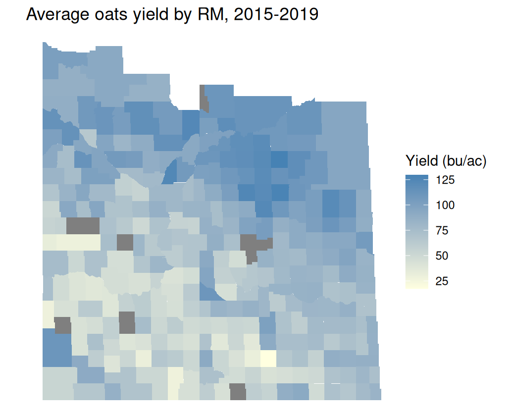
(a) Build a table of the average oats yield in each RM over 2015 to 2019.
(b) Join it to the boundaries and map it, with a title and a legend label.
Answer
Pseudocode
read sask_rms.geojson
read rm_yields_1990_2025.csv

keep the rows where the crop is oats and the year is from 2015 to 2019
for each RM, work out the average yield over those years

join the averages onto the boundaries

map the RMs with fill set by the average yield
  title it and label the legend
R code
rms <-st_read("data/sask_rms.geojson", quiet =TRUE) |>clean_names() |>mutate(rmno =as.numeric(rmno))yields <-read_csv("data/rm_yields_1990_2025.csv", show_col_types =FALSE) |>clean_names()##(a) the average over 2015-2019avg <- yields |>filter(crop =="Oats", year >=2015, year <=2019) |>summarise(mean_yield =mean(yield), .by = rm)##(b) attach it to the boundariesrms_oats <-left_join(rms, avg, by =c("rmno"="rm"))
> rms <- st_read("data/sask_rms.geojson", quiet = TRUE) |>
+   clean_names() |>
+   mutate(rmno = as.numeric(rmno))
>
> yields <- read_csv("data/rm_yields_1990_2025.csv", show_col_types = FALSE) |>
+   clean_names()
>
> ##(a) the average over 2015-2019
> avg <- yields |>
+   filter(crop == "Oats", year >= 2015, year <= 2019) |>
+   summarise(mean_yield = mean(yield), .by = rm)
>
> ##(b) attach it to the boundaries
> rms_oats <- left_join(rms, avg, by = c("rmno" = "rm"))
This question uses sask_rms.geojson and rm_yields_1990_2025.csv.
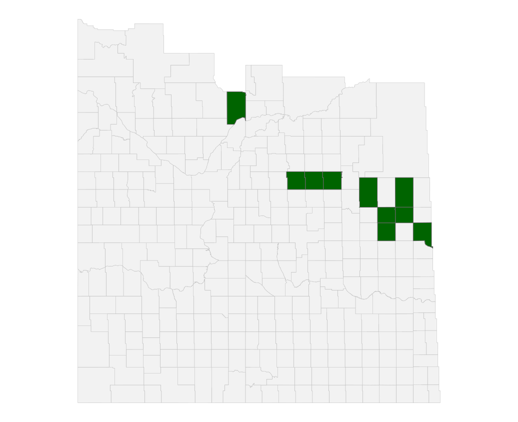
(a) Find the ten RMs with the highest average canola yield over 2020 to 2025.
(b) Map the province in grey with those ten shaded.
(c) In a comment: is a map the best way to show a top-ten list? Say why or why not.
Answer
Pseudocode
read sask_rms.geojson
read rm_yields_1990_2025.csv

keep the canola rows from 2020 onwards
for each RM, work out the average yield
sort from highest to lowest and keep the first ten

pull those ten RMs out of the boundaries

map all the RMs in grey
  draw the ten on top in a strong colour

in a comment, say whether a map is the right chart here
R code
rms <-st_read("data/sask_rms.geojson", quiet =TRUE) |>clean_names() |>mutate(rmno =as.numeric(rmno))yields <-read_csv("data/rm_yields_1990_2025.csv", show_col_types =FALSE) |>clean_names()##(a) the top ten RMstop10 <- yields |>filter(crop =="Canola", year >=2020, year <=2025) |>summarise(mean_yield =mean(yield, na.rm =TRUE), .by = rm) |>slice_max(mean_yield, n =10)top10##(b) those ten, as boundariestop_rms <-filter(rms, rmno %in% top10$rm)
ggplot() +geom_sf(data = rms, fill ="grey95", colour ="grey75", linewidth =0.1) +geom_sf(data = top_rms, fill ="darkgreen", colour ="grey40") +theme_void()
(c) A map answers “where are they”, which a bar chart cannot. It does not answer “how much better are they”, because the shading is the same for first and tenth. If the ranking is the point, a bar chart is better; if clustering is the point, the map is.
Question 20
This question uses sask_rms.geojson. A table of four elevators is given in the question.
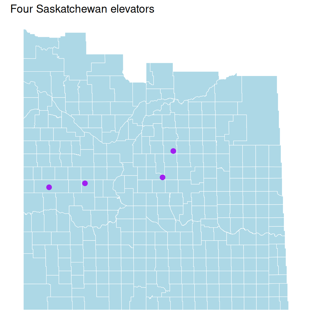
(a) Build this table in R and turn it into spatial data. The coordinates are degrees.
Elevator
Longitude
Latitude
Rosetown
-108.00
51.55
Watrous
-105.47
51.67
Kindersley
-109.17
51.47
Humboldt
-105.12
52.20
(b) Map the RM boundaries with the four elevators drawn on top as points.
(c) Give the map a title.
Answer
Pseudocode
read sask_rms.geojson

make a table of the four elevators with their longitude and latitude
turn it into spatial data, saying which columns are the coordinates
  and that they are in degrees

map the RMs, then draw the elevators on top as points
  title it
R code
rms <-st_read("data/sask_rms.geojson", quiet =TRUE) |>clean_names()##(a) the four elevators as a plain tableelevators <-data.frame(elevator =c("Rosetown", "Watrous", "Kindersley", "Humboldt"),lon =c(-108.00, -105.47, -109.17, -105.12),lat =c(51.55, 51.67, 51.47, 52.20))##Turn the coordinate columns into point geometry, in degreeselevators_sf <-st_as_sf(elevators, coords =c("lon", "lat"), crs =4326)elevators_sf
> rms <- st_read("data/sask_rms.geojson", quiet = TRUE) |>
+   clean_names()
>
> ##(a) the four elevators as a plain table
> elevators <- data.frame(
+   elevator = c("Rosetown", "Watrous", "Kindersley", "Humboldt"),
+   lon = c(-108.00, -105.47, -109.17, -105.12),
+   lat = c(51.55, 51.67, 51.47, 52.20)
+ )
>
> ##Turn the coordinate columns into point geometry, in degrees
> elevators_sf <- st_as_sf(elevators, coords = c("lon", "lat"), crs = 4326)
>
> elevators_sf
Simple feature collection with 4 features and 1 field
Geometry type: POINT
Dimension:     XY
Bounding box:  xmin: -109.17 ymin: 51.47 xmax: -105.12 ymax: 52.2
Geodetic CRS:  WGS 84
    elevator              geometry
1   Rosetown    POINT (-108 51.55)
2    Watrous POINT (-105.47 51.67)
3 Kindersley POINT (-109.17 51.47)
4   Humboldt  POINT (-105.12 52.2)
##(b) and (c) the polygons, then the points on topggplot() +geom_sf(data = rms, fill ="lightblue", colour ="white") +geom_sf(data = elevators_sf, colour ="purple", size =2.5) +labs(title ="Four Saskatchewan elevators") +theme_void()
Section 3 — Spatial operations
For each of these you write pseudocode in Part 1 and an R script in Part 2. The RM and risk zone files arrive in degrees and the raster is in UTM metres, so any question combining them with the raster needs a transform first, as the chapter does. For areas and distances on the vector layers alone you do not need one – sf measures on the curved earth and returns metres either way. Your test will name a different RM, zone or crop from the one below.
Question 21
This question uses sask_rms.geojson.
(a) Report the area of the RM of Redberry in square kilometres.
(b) Calculate the area of every RM in Saskatchewan and report the median.
(c) Report how many RMs are larger than Redberry.
Answer
Pseudocode
read sask_rms.geojson

pull out the row for REDBERRY
  calculate its area and convert from square metres to square kilometres

calculate the area of all 296 RMs
  report the median
  count how many of them are larger than Redberry
R code
rms <-st_read("data/sask_rms.geojson", quiet =TRUE) |>clean_names()##(a) one RMredberry <-filter(rms, rmnm =="REDBERRY")redberry_km2 <-as.numeric(st_area(redberry)) /1e6redberry_km2##(b) an area column for all of themrms <- rms |>mutate(km2 =as.numeric(st_area(geometry)) /1e6)median(rms$km2)##(c) how many are biggersum(rms$km2 > redberry_km2)
> rms <- st_read("data/sask_rms.geojson", quiet = TRUE) |>
+   clean_names()
>
> ##(a) one RM
> redberry <- filter(rms, rmnm == "REDBERRY")
> redberry_km2 <- as.numeric(st_area(redberry)) / 1e6
> redberry_km2
[1] 1103.116
>
> ##(b) an area column for all of them
> rms <- rms |>
+   mutate(km2 = as.numeric(st_area(geometry)) / 1e6)
>
> median(rms$km2)
[1] 853.0342
>
> ##(c) how many are bigger
> sum(rms$km2 > redberry_km2)
[1] 62
Question 22
This question uses sask_rms.geojson and sk_risk_zones.geojson.
(a) Calculate the total area of the RM of Leask, in square kilometres.
(b) Report which risk zones Leask falls in.
(c) Calculate the area of Leask that is in each risk zone, in square kilometres.
Answer
Pseudocode
read sask_rms.geojson and sk_risk_zones.geojson

pull out the row for LEASK
  calculate its area and convert from square metres to square kilometres

find which risk zones it shares ground with, and report their numbers

cut Leask at the zone boundaries, giving one piece per zone
  calculate the area of each piece in square kilometres
R code
rms <-st_read("data/sask_rms.geojson", quiet =TRUE) |>clean_names()zones <-st_read("data/sk_risk_zones.geojson", quiet =TRUE)leask <-filter(rms, rmnm =="LEASK")##(a) the area of the whole RMas.numeric(st_area(leask)) /1e6##(b) which zones it falls inhit <-st_intersects(leask, zones)zones$risk_zone[hit[[1]]]##(c) cut it at the zone boundaries and measure the piecespieces <-st_intersection(leask, zones) |>mutate(km2 =as.numeric(st_area(geometry)) /1e6)st_drop_geometry(pieces) |>select(rmnm, risk_zone, km2)##The pieces add to very nearly the area from part (a): the two layers were##drawn separately, so their edges do not line up perfectly and the overlay##does not close exactly.
> rms <- st_read("data/sask_rms.geojson", quiet = TRUE) |>
+   clean_names()
> zones <- st_read("data/sk_risk_zones.geojson", quiet = TRUE)
>
> leask <- filter(rms, rmnm == "LEASK")
>
> ##(a) the area of the whole RM
> as.numeric(st_area(leask)) / 1e6
[1] 1494.25
>
> ##(b) which zones it falls in
> hit <- st_intersects(leask, zones)
> zones$risk_zone[hit[[1]]]
[1] 18 22
>
> ##(c) cut it at the zone boundaries and measure the pieces
> pieces <- st_intersection(leask, zones) |>
+   mutate(km2 = as.numeric(st_area(geometry)) / 1e6)
Warning: attribute variables are assumed to be spatially constant throughout all geometries
>
> st_drop_geometry(pieces) |> select(rmnm, risk_zone, km2)
     rmnm risk_zone        km2
1   LEASK        18 1470.51813
1.1 LEASK        22   23.72144
>
> ##The pieces add to very nearly the area from part (a): the two layers were
> ##drawn separately, so their edges do not line up perfectly and the overlay
> ##does not close exactly.
Question 23
This question uses sask_rms.geojson and sk_risk_zones.geojson.
(a) Report how many RMs are (at least partly) in risk zone 12.
(b) Report the fraction of each of those RMs that is contained within risk zone 12. For some RMs this will be 1 – they are completely inside the zone. For others it will be between 0 and 1.
(c) In a comment: explain the difference between the two answers you would get from st_intersects() and st_intersection().
Answer
Pseudocode
read sask_rms.geojson and sk_risk_zones.geojson

pull out risk zone 12
find every RM that shares any ground with it, and count them

calculate the area of each of those RMs

cut those RMs at the zone boundary
  calculate the area of each piece that is left

divide the clipped area by the whole area to get the fraction in the zone

in a comment, explain what each of the two operations returned
R code
rms <-st_read("data/sask_rms.geojson", quiet =TRUE) |>clean_names()zones <-st_read("data/sk_risk_zones.geojson", quiet =TRUE)zone12 <-filter(zones, risk_zone ==12)##(a) which RMs are in the zone at allhit <-st_intersects(zone12, rms)in_zone <- rms[hit[[1]], ]nrow(in_zone)##The area of each whole RMin_zone <- in_zone |>mutate(whole_km2 =as.numeric(st_area(geometry)) /1e6)##(b) cut them at the zone boundary and measure what is leftclipped <-st_intersection(in_zone, zone12) |>mutate(clipped_km2 =as.numeric(st_area(geometry)) /1e6)##The fraction of each RM that falls in the zonefractions <- clipped |>st_drop_geometry() |>mutate(fraction =round(clipped_km2 / whole_km2, 3)) |>select(rmnm, whole_km2, clipped_km2, fraction) |>arrange(fraction)fractions##Most of these RMs are only partly in the zone. The ones that are wholly##inside come out at 0.997 or so rather than exactly 1: the RM and the zone##boundaries were drawn separately, so they do not line up to the metre.##(c) st_intersects() returned the row numbers of the matching RMs, and we##used those to select whole polygons. st_intersection() cut them at the##zone boundary, so each piece is only the part inside the zone.
> rms <- st_read("data/sask_rms.geojson", quiet = TRUE) |>
+   clean_names()
> zones <- st_read("data/sk_risk_zones.geojson", quiet = TRUE)
>
> zone12 <- filter(zones, risk_zone == 12)
>
> ##(a) which RMs are in the zone at all
> hit <- st_intersects(zone12, rms)
> in_zone <- rms[hit[[1]], ]
> nrow(in_zone)
[1] 26
>
> ##The area of each whole RM
> in_zone <- in_zone |>
+   mutate(whole_km2 = as.numeric(st_area(geometry)) / 1e6)
>
> ##(b) cut them at the zone boundary and measure what is left
> clipped <- st_intersection(in_zone, zone12) |>
+   mutate(clipped_km2 = as.numeric(st_area(geometry)) / 1e6)
Warning: attribute variables are assumed to be spatially constant throughout all geometries
>
> ##The fraction of each RM that falls in the zone
> fractions <- clipped |>
+   st_drop_geometry() |>
+   mutate(fraction = round(clipped_km2 / whole_km2, 3)) |>
+   select(rmnm, whole_km2, clipped_km2, fraction) |>
+   arrange(fraction)
>
> fractions
                   rmnm whole_km2 clipped_km2 fraction
1  LAST MOUNTAIN VALLEY  886.1961     4.97089    0.006
2               VANSCOY  905.1525    17.46699    0.019
3           CORMAN PARK 2273.8167    49.30869    0.022
4                COTEAU  931.1810    25.95801    0.028
5               BLUCHER  849.6002    24.45821    0.029
6            WOOD CREEK  850.3393    25.39241    0.030
7                MORRIS  900.3726    35.06179    0.039
8        FERTILE VALLEY 1028.2150    49.53829    0.048
9               MARQUIS  835.3111    44.30045    0.053
10             MCKILLOP  680.6158    41.96840    0.062
11               CANAAN  554.7326    44.45083    0.080
12           LOST RIVER  568.2368    50.41797    0.089
13              BIG ARM  819.4090    76.62938    0.094
14             MONTROSE  902.1006   172.55750    0.191
15           MAPLE BUSH  967.8526   834.06476    0.862
16                HURON  851.3666   774.44501    0.910
17                 RUDY  857.7118   780.68842    0.910
18             DUFFERIN  994.6178   913.09589    0.918
19             LOREBURN 1060.1372   974.44037    0.919
20              DUNDURN  872.0869   837.18824    0.960
21                CRAIK  892.0552   865.35853    0.970
22               SARNIA  958.7008   932.22197    0.972
23            ARM RIVER  729.8155   727.80510    0.997
24             ROSEDALE  945.4131   944.21507    0.999
25             MCCRANEY  970.3799   969.03575    0.999
26              WILLNER  852.6312   852.63121    1.000
>
> ##Most of these RMs are only partly in the zone. The ones that are wholly
> ##inside come out at 0.997 or so rather than exactly 1: the RM and the zone
> ##boundaries were drawn separately, so they do not line up to the metre.
>
> ##(c) st_intersects() returned the row numbers of the matching RMs, and we
> ##used those to select whole polygons. st_intersection() cut them at the
> ##zone boundary, so each piece is only the part inside the zone.
Question 24
This question uses sask_rms.geojson, sk_risk_zones.geojson and rm_yields_1990_2025.csv.
(a) Clip the RM boundaries to risk zone 12, so only the land inside the zone is left.
(b) Join the 2023 canola yields onto those RMs, and report the average yield across the zone.
(c) Map the clipped RMs with fill set by yield, and the zone boundary drawn over them.
Answer
Pseudocode
read sask_rms.geojson and sk_risk_zones.geojson
read rm_yields_1990_2025.csv

pull out risk zone 12
cut the RMs at the zone boundary, keeping only the part inside

keep the yield rows where the crop is canola and the year is 2023
join them onto the clipped RMs, matching RM number to RM number

average the yields across the RMs in the zone

map the clipped RMs with fill set by yield, and draw the zone boundary on top
R code
rms <-st_read("data/sask_rms.geojson", quiet =TRUE) |>clean_names() |>mutate(rmno =as.numeric(rmno))zones <-st_read("data/sk_risk_zones.geojson", quiet =TRUE)yields <-read_csv("data/rm_yields_1990_2025.csv", show_col_types =FALSE) |>clean_names()zone12 <-filter(zones, risk_zone ==12)##(a) cut the RMs at the zone boundaryclipped <-st_intersection(rms, zone12)nrow(clipped)##(b) attach the 2023 canola yields and average themcanola <-filter(yields, crop =="Canola", year ==2023)zone_yields <-left_join(clipped, canola, by =c("rmno"="rm"))mean(zone_yields$yield, na.rm =TRUE)##For comparison, the provincial average that yearmean(canola$yield, na.rm =TRUE)
> rms <- st_read("data/sask_rms.geojson", quiet = TRUE) |>
+   clean_names() |>
+   mutate(rmno = as.numeric(rmno))
>
> zones <- st_read("data/sk_risk_zones.geojson", quiet = TRUE)
>
> yields <- read_csv("data/rm_yields_1990_2025.csv", show_col_types = FALSE) |>
+   clean_names()
>
> zone12 <- filter(zones, risk_zone == 12)
>
> ##(a) cut the RMs at the zone boundary
> clipped <- st_intersection(rms, zone12)
Warning: attribute variables are assumed to be spatially constant throughout all geometries
> nrow(clipped)
[1] 26
>
> ##(b) attach the 2023 canola yields and average them
> canola <- filter(yields, crop == "Canola", year == 2023)
> zone_yields <- left_join(clipped, canola, by = c("rmno" = "rm"))
>
> mean(zone_yields$yield, na.rm = TRUE)
[1] 24.48462
>
> ##For comparison, the provincial average that year
> mean(canola$yield, na.rm = TRUE)
[1] 33.88097
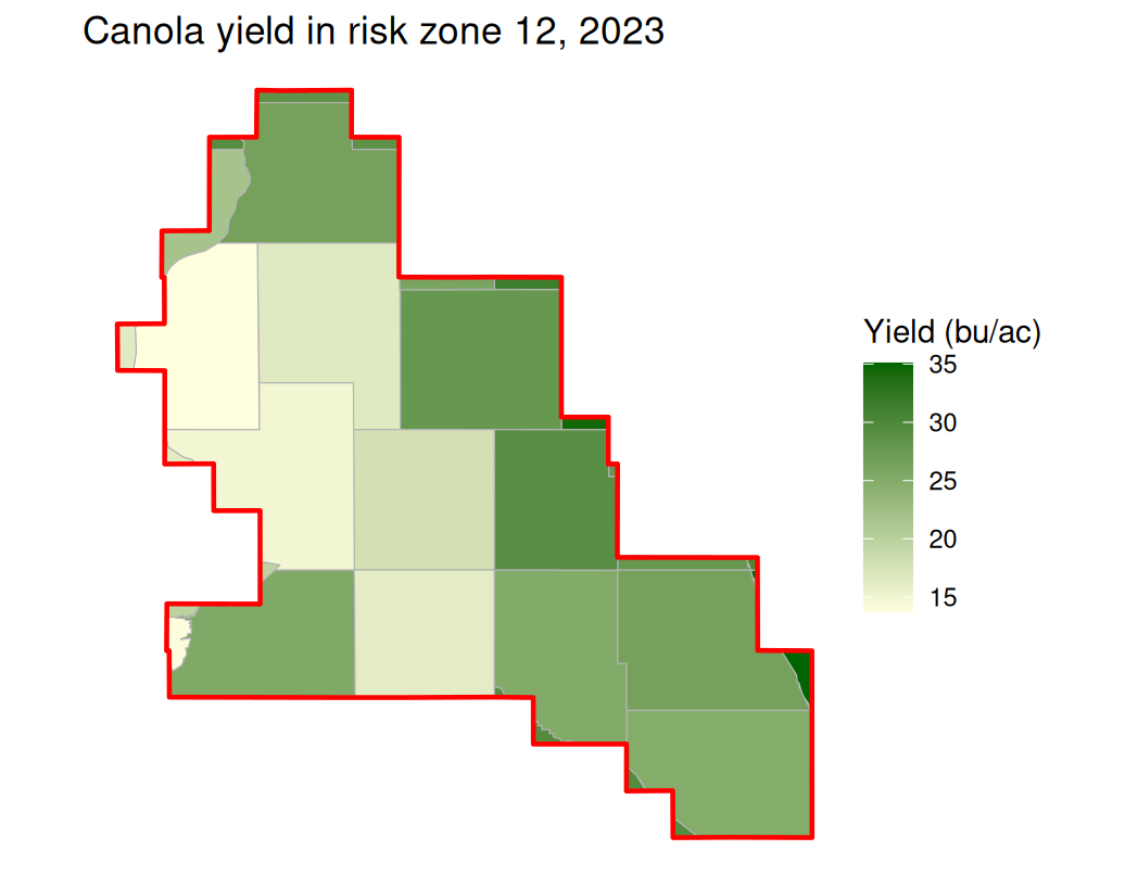
ggplot() +geom_sf(data = zone_yields, aes(fill = yield), colour ="grey70") +geom_sf(data = zone12, fill =NA, colour ="red", linewidth =0.8) +scale_fill_gradient(low ="lightyellow", high ="darkgreen",name ="Yield (bu/ac)") +labs(title ="Canola yield in risk zone 12, 2023") +theme_void()
Question 25
This question uses sask_rms.geojson and sk_risk_zones.geojson.
(a) Report how many RMs fall entirely inside risk zone 16.
(b) Report how many share any ground with it.
(c) Map the zone boundary in red, the RMs wholly inside it in dark blue, and the rest of those sharing ground in light blue.
Answer
Pseudocode
read sask_rms.geojson and sk_risk_zones.geojson

pull out risk zone 16

find the RMs that fall wholly within the zone, and count them
find the RMs that share any ground with the zone, and count them

map the zone boundary with both sets of RMs drawn in different colours
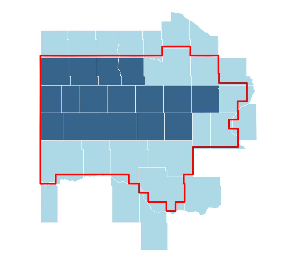
ggplot() +geom_sf(data = touching, fill ="lightblue", colour ="white") +geom_sf(data = inside, fill ="steelblue4", colour ="white") +geom_sf(data = zone16, fill =NA, colour ="red", linewidth =1) +theme_void()
Question 26
This question uses aci_slice_2023.tif, aci_crop_classes.csv and sask_rms.geojson.
(a) Cut the crop inventory raster down to the RM of Blaine Lake, in two steps.
(b) Report how many cells are missing after each step.
(c) In a comment: explain why the two steps give different numbers.
Answer
Pseudocode
read aci_slice_2023.tif
read sask_rms.geojson and put it in the raster's CRS

pull out the row for BLAINE LAKE

trim the raster to the RM's bounding box
  report how many cells are missing

blank out the cells outside the RM itself
  report how many cells are missing now

in a comment, explain the difference
R code
aci <-rast("data/aci_slice_2023.tif")rms <-st_read("data/sask_rms.geojson", quiet =TRUE) |>clean_names() |>st_transform(st_crs(aci))blaine <-filter(rms, rmnm =="BLAINE LAKE")##(a) step one: trim to the bounding boxaci_box <-crop(aci, blaine)global(is.na(aci_box), "sum")##step two: blank what is outside the RMaci_rm <-mask(aci_box, blaine)global(is.na(aci_rm), "sum")##(c) In this raster, crop() only cuts whole rows and columns off the##outside, so nothing is missing -- the RM lies entirely inside the slice. mask() sets the cells outside the polygon to NA. The grid is##the same size either way -- only the values change.
> aci <- rast("data/aci_slice_2023.tif")
> rms <- st_read("data/sask_rms.geojson", quiet = TRUE) |>
+   clean_names() |>
+   st_transform(st_crs(aci))
>
> blaine <- filter(rms, rmnm == "BLAINE LAKE")
>
> ##(a) step one: trim to the bounding box
> aci_box <- crop(aci, blaine)
> global(is.na(aci_box), "sum")
               sum
aci_2023_sk_v4   0
>
> ##step two: blank what is outside the RM
> aci_rm <- mask(aci_box, blaine)
> global(is.na(aci_rm), "sum")
                  sum
aci_2023_sk_v4 767373
>
> ##(c) In this raster, crop() only cuts whole rows and columns off the
> ##outside, so nothing is missing -- the RM lies entirely inside the slice. mask() sets the cells outside the polygon to NA. The grid is
> ##the same size either way -- only the values change.
Question 27
This question uses aci_slice_2023.tif, aci_crop_classes.csv and sask_rms.geojson.
(a) Report what share of the RM of Redberry is canola, which is class 153.
(b) Report the five largest shares. You can report these by their numeric code – frac_153 and so on – without converting the codes to crop names.
(c) Convert the canola share from part (a) to acres. One acre is 4,046.86 square metres.
Answer
Pseudocode
read aci_slice_2023.tif, aci_crop_classes.csv and sask_rms.geojson
put the boundaries in the raster's CRS

pull out the row for REDBERRY

work out what share of the RM each class covers
  the result has one column per class, named frac_ then the class code

read the canola share off the column for the canola code
sort the shares and report the five largest, by their column names

multiply the canola share by the area of the RM, then divide by 4,046.86
  to turn square metres into acres
R code
aci <-rast("data/aci_slice_2023.tif")classes <-read_csv("data/aci_crop_classes.csv", show_col_types =FALSE)rms <-st_read("data/sask_rms.geojson", quiet =TRUE) |>clean_names() |>st_transform(st_crs(aci))redberry <-filter(rms, rmnm =="REDBERRY")##The share of the RM covered by each class. One column per class,##named frac_ then the class code.shares <-exact_extract(aci, redberry, "frac", progress =FALSE)##(a) canola is class 153, so the column is frac_153canola_share <- shares$frac_153100* canola_share##(b) the five largest shares, by column nameround(100*sort(unlist(shares), decreasing =TRUE)[1:5], 1)
> aci <- rast("data/aci_slice_2023.tif")
> classes <- read_csv("data/aci_crop_classes.csv", show_col_types = FALSE)
> rms <- st_read("data/sask_rms.geojson", quiet = TRUE) |>
+   clean_names() |>
+   st_transform(st_crs(aci))
>
> redberry <- filter(rms, rmnm == "REDBERRY")
>
> ##The share of the RM covered by each class. One column per class,
> ##named frac_ then the class code.
> shares <- exact_extract(aci, redberry, "frac", progress = FALSE)
>
> ##(a) canola is class 153, so the column is frac_153
> canola_share <- shares$frac_153
> 100 * canola_share
[1] 25.22767
>
> ##(b) the five largest shares, by column name
> round(100 * sort(unlist(shares), decreasing = TRUE)[1:5], 1)
frac_153 frac_146  frac_50  frac_20 frac_220
    25.2     19.9      9.8      8.1      7.1
##(c) the same share, converted to acresrm_area_m2 <-as.numeric(st_area(redberry))canola_share * rm_area_m2 /4046.86
> ##(c) the same share, converted to acres
> rm_area_m2 <- as.numeric(st_area(redberry))
>
> canola_share * rm_area_m2 / 4046.86
[1] 69027.73
Question 28
This question uses sask_rms.geojson, and aci_slice_2023.tif only to borrow its CRS – a buffer needs the layer on a flat grid, so that 25 km means 25 km in every direction.
(a) Draw a 25 km buffer around the RM of Redberry and report its area in square kilometres.
(b) Report how much larger the buffer is than Redberry itself.
(c) Map Redberry, the buffer around it, and the RMs the buffer reaches.
Answer
Pseudocode
read sask_rms.geojson and put it in the same CRS as the raster

pull out the Redberry row
grow it by 25 km in every direction
  calculate the area of the buffer, and of Redberry itself
  report the difference

find the RMs that share ground with the buffer

map the buffer, those RMs, and Redberry on top
R code
rms <-st_read("data/sask_rms.geojson", quiet =TRUE) |>clean_names() |>st_transform(st_crs(rast("data/aci_slice_2023.tif")))redberry <-filter(rms, rmnm =="REDBERRY")##(a) grow it by 25 kmbuffer <-st_buffer(redberry, 25000)as.numeric(st_area(buffer)) /1e6##(b) how much bigger than the RM itselfas.numeric(st_area(buffer) -st_area(redberry)) /1e6##(c) the RMs the buffer reachesreached <- rms[lengths(st_intersects(rms, buffer)) >0, ]nrow(reached)
> rms <- st_read("data/sask_rms.geojson", quiet = TRUE) |>
+   clean_names() |>
+   st_transform(st_crs(rast("data/aci_slice_2023.tif")))
>
> redberry <- filter(rms, rmnm == "REDBERRY")
>
> ##(a) grow it by 25 km
> buffer <- st_buffer(redberry, 25000)
> as.numeric(st_area(buffer)) / 1e6
[1] 6425.817
>
> ##(b) how much bigger than the RM itself
> as.numeric(st_area(buffer) - st_area(redberry)) / 1e6
[1] 5318.518
>
> ##(c) the RMs the buffer reaches
> reached <- rms[lengths(st_intersects(rms, buffer)) > 0, ]
> nrow(reached)
[1] 12
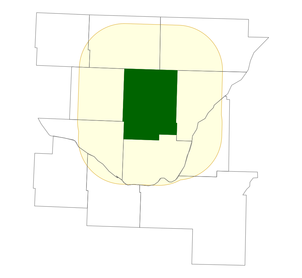
ggplot() +geom_sf(data = buffer, fill ="lightyellow", colour ="goldenrod") +geom_sf(data = reached, fill =NA, colour ="grey40") +geom_sf(data = redberry, fill ="darkgreen", colour ="darkgreen") +theme_void()
Question 29
This question uses sask_rms.geojson.
(a) Report how far the RM of Rosedale is from the RM of Leask, in kilometres.
(b) Report which RM is furthest from Rosedale, and how far away it is.
(c) Map Rosedale and that furthest RM, with every other RM in grey behind them.
Answer
Pseudocode
read sask_rms.geojson and put it in the same CRS as the raster,
  so the distances come back in metres

pull out the Rosedale row and the Leask row
  measure the distance between them, and convert to kilometres

measure the distance from Rosedale to every RM
  find the largest, and which RM it belongs to

map all the RMs in grey, with Rosedale and that RM drawn on top
R code
rms <-st_read("data/sask_rms.geojson", quiet =TRUE) |>clean_names() |>mutate(rmno =as.numeric(rmno))rosedale <-filter(rms, rmno ==283)##(a) one pair, in kilometresleask <-filter(rms, rmnm =="LEASK")as.numeric(st_distance(rosedale, leask)) /1000##(b) the furthest RM from Rosedaled <-as.numeric(st_distance(rosedale, rms)) /1000furthest <- rms[which.max(d), ]furthest$rmnmmax(d)
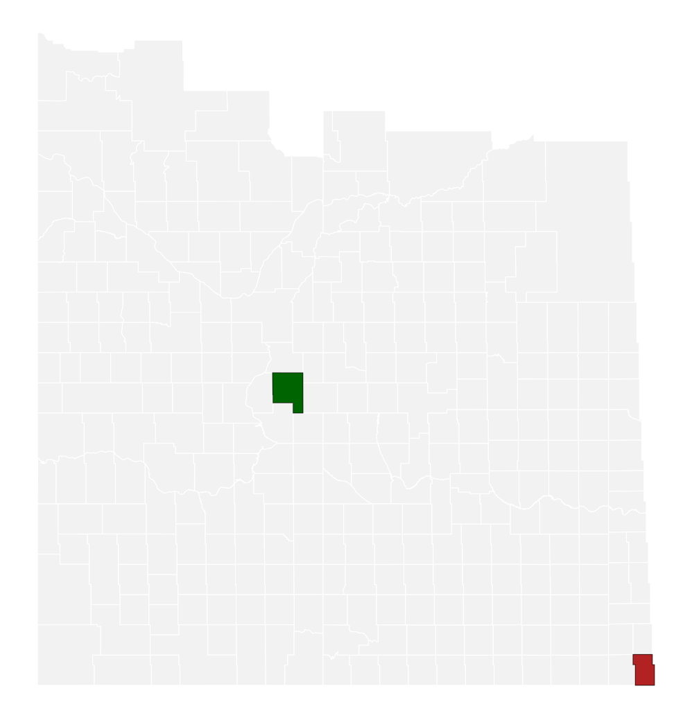
ggplot() +geom_sf(data = rms, fill ="grey95", colour ="white") +geom_sf(data = rosedale, fill ="darkgreen") +geom_sf(data = furthest, fill ="firebrick") +theme_void()
Question 30
This question uses sask_rms.geojson and sk_quarters.geojson.
(a) Report how many quarter sections fall in the RM of Leask.
(b) Report the total area of those quarters in square kilometres, and the area of the RM itself.
(c) Map the quarters with the RM boundary drawn over them.
Answer
Pseudocode
read sask_rms.geojson and sk_quarters.geojson

pull out the Leask row
keep the quarters whose RM name is Leask
  count them
  add up their areas, and compare with the area of the RM

map those quarters with the RM boundary on top
R code
rms <-st_read("data/sask_rms.geojson", quiet =TRUE) |>clean_names()quarters <-st_read("data/sk_quarters.geojson", quiet =TRUE) |>clean_names()leask <-filter(rms, rmnm =="LEASK")##(a) the quarters in that RMleask_q <-filter(quarters, rmnm =="LEASK")nrow(leask_q)##(b) their total area, against the area of the RMsum(as.numeric(st_area(leask_q))) /1e6as.numeric(st_area(leask)) /1e6
> rms <- st_read("data/sask_rms.geojson", quiet = TRUE) |>
+   clean_names()
>
> quarters <- st_read("data/sk_quarters.geojson", quiet = TRUE) |>
+   clean_names()
>
> leask <- filter(rms, rmnm == "LEASK")
>
> ##(a) the quarters in that RM
> leask_q <- filter(quarters, rmnm == "LEASK")
> nrow(leask_q)
[1] 2277
>
> ##(b) their total area, against the area of the RM
> sum(as.numeric(st_area(leask_q))) / 1e6
[1] 1467.882
> as.numeric(st_area(leask)) / 1e6
[1] 1494.25
ggplot() +geom_sf(data = leask_q, fill ="honeydew", colour ="grey60",linewidth =0.1) +geom_sf(data = leask, fill =NA, colour ="red", linewidth =1) +theme_void()