model4 <- lm(Canola ~ Precip_May_Aug_mm + Days_Above_30 + latitude + soil_zone,
             data = canola)
> model4 <- lm(Canola ~ Precip_May_Aug_mm + Days_Above_30 + latitude + soil_zone,
+ data = canola)A major benefit of including multiple variables in a model is that we will obtain much better predictions than we would with a single variable. In this chapter, we go over how to assess the quality of a model’s predictions, and how to avoid being misled by a model that looks good on the surface but will deliver bad predictions.
Recall that a regression model is
\[ y_i = \beta_0 + \beta_1 x_{1i} + \beta_2 x_{2i} + \beta_3 x_{3i} + \ldots + \varepsilon_i \]
Once we estimate the model, we have a set of coefficients \(\hat{\beta}_0, \hat{\beta}_1, \hat{\beta}_2, \hat{\beta}_3, \ldots\) that we can use to make predictions for the response variable \(y\). Note that we use a hat to indicate that these are estimates of the true coefficients – so \(\hat{\beta}_1\) is our estimate of the true coefficient \(\beta_1\).
We can then decompose the response variable into two parts: the part that is predicted by the model, and the part that is not. The predicted part is called the fitted value \(\hat{y}_i\), and the part that is not predicted is called the residual \(\hat{\varepsilon}_i\): \[ y_i = \underbrace{\hat{\beta}_0 + \hat{\beta}_1 x_{1i} + \hat{\beta}_2 x_{2i} + \hat{\beta}_3 x_{3i} + \ldots}_{\text{Fitted value}} + \underbrace{\hat{\varepsilon}_i}_{\text{Residual}} \] We can often just write the fitted value as \(\hat{y_i}\) such that the residual is simply the difference between the observed value and the fitted value: \[ \hat{\varepsilon}_i = y_i - \hat{y}_i \]
A positive residual means that the actual response variable for row \(i\) was above what the model predicted. For example, in a yield model, a positive residual means the field yielded more than the model predicted, and a negative residual means it yielded less.
Let’s return to our model of canola yields across RMs that we built in Chapter 26. Recall that this model was:
model4 <- lm(Canola ~ Precip_May_Aug_mm + Days_Above_30 + latitude + soil_zone,
data = canola)> model4 <- lm(Canola ~ Precip_May_Aug_mm + Days_Above_30 + latitude + soil_zone,
+ data = canola)| Term | Estimate | Std. Error | t value | p value |
|---|---|---|---|---|
| Intercept | 26.4649 | 8.0503 | 3.29 | 0.001 |
| May to Aug precip (mm) | 0.0077 | 0.0021 | 3.61 | <0.001 |
| Days above 30 degrees | -0.7296 | 0.0227 | -32.10 | <0.001 |
| Latitude | 0.2612 | 0.1582 | 1.65 | 0.099 |
| Soil zone: Dark Brown | 2.7251 | 0.3980 | 6.85 | <0.001 |
| Soil zone: Grey/Black | 4.0360 | 0.5358 | 7.53 | <0.001 |
Take RM 1 (Argyle) in 2024. It is in the Dark Brown soil zone, at a latitude of 49.13, and that season it received 294.6 mm of rain between May and August with 6 days above 30 °C. Putting those numbers into the model gives the fitted value:
\[ \hat{y} = \underbrace{26.4649}_{\text{intercept}} + \underbrace{294.6 \times 0.0077}_{\text{precipitation}} + \underbrace{6 \times (-0.7296)}_{\text{hot days}} + \underbrace{49.13 \times 0.2612}_{\text{latitude}} + \underbrace{2.7251}_{\text{Dark Brown}} = 39.9 \]
Argyle actually yielded 36.4 bu/ac that year, so the residual is
\[ \hat{\varepsilon} = \underbrace{36.4}_{\text{actual}} - \underbrace{39.9}_{\text{fitted}} = -3.5 \]
This is to say, the model expected about three and a half bushels more than the RM delivered.
Fortunately, R will easily compute the fitted vales and residuals for every observation in our model using the fitted() and resid() functions.
canola$predicted <- fitted(model4)
canola$residual  <- resid(model4)

head(canola[, c("RM_Name", "Year", "Canola", "predicted", "residual")])
> canola$predicted <- fitted(model4)
> canola$residual <- resid(model4)
>
> head(canola[, c("RM_Name", "Year", "Canola", "predicted", "residual")])
# A tibble: 6 × 5
RM_Name Year Canola predicted residual
<chr> <dbl> <dbl> <dbl> <dbl>
1 Argyle 2015 28.6 39.1 -10.4
2 Mount Pleasant 2015 29.4 39.1 -9.60
3 Enniskillen 2015 31.0 36.3 -5.29
4 Coalfields 2015 25.4 25.9 -0.503
5 Estevan 2015 30.6 25.9 4.71
6 Cambria 2015 31.4 25.9 5.53 A good practice is to plot the residuals of the model against the values of fitted values. This can reveal if there are outliers that are not well predicted by the model. By construction, the residuals will always average zero, so they should be scattered around a horizontal line at zero. If the model is missing in a systematic way, the residuals will show a pattern rather than being randomly scattered.
ggplot(canola, aes(x = predicted, y = residual)) +
  geom_point(alpha = 0.2) +
  geom_hline(yintercept = 0, linetype = "dashed") +
  labs(x = "Fitted value (bu/ac)", y = "Residual (bu/ac)") +
  theme_minimal()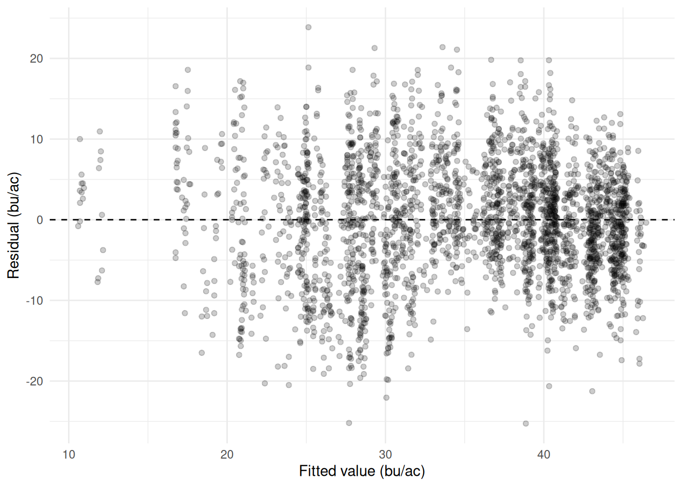
We can now return to the definition of \(R^2\) from Section 24.4. Recall, that we had defined the \(R^2\) as the proportion of the variance in the response variable that is predictable from the predictor variables. We can now be a bit more precise. First, consider what our best prediction of the response variable is if we do not use any predictors at all. In that case, our best guess for every observation is simply the mean of the response variable. The errors from such a model would be the difference between the actual values and the mean of the response variable.
If we simply add up these errors the result will be zero, because deviations from the mean always cancel out – that is what the mean is. If we square these errors, it gives us a measure of the total variability in the response variable. We call this the “Total Sum of Squares”: \[ \text{SST} = \sum_{i=1}^{n} (y_i - \bar{y})^2 \] We can note that the SST is essentially the variance of the response variable multiplied by \(n-1\).
Now consider the errors from our model. These are the residuals, which are the difference between the actual values and the fitted values. If we square these residuals and add them up, we get the “Sum of Squared Errors” (SSE), which is a measure of the variance between what our model predicts and the actual values: \[ \text{SSE} = \sum_{i=1}^{n} (y_i - \hat{y}_i)^2 \]
We can now formally define the \(R^2\) as:
\[ R^2 = 1 - \frac{\text{SSE}}{\text{SST}} \]
Note that if \(SSE=SST\) then our model does no better at predicting the response variable than simply guessing the mean every time, and \(R^2=0\). If \(SSE=0\) then our model predicts the response variable perfectly, and \(R^2=1\). The higher the \(R^2\), the greater the proportion of variation in the response variable the model accounts for.
Measured this way – on the same observations the model was fitted on, with an intercept in the model – \(R^2\) cannot fall outside 0 and 1. That guarantee does not survive being applied to data the model has not seen, and later in this chapter we will compute an \(R^2\) that comes out negative.
The \(R^2\) value can tell us how well our model predicts the data that are used in the model – an \(R^2\) of 1 denotes a perfect prediction, an \(R^2\) of 0 means no improvement over guessing the mean every time. There are two other measures of predictive accuracy that are frequently used to validate model performance: mean absolute error (MAE) and root mean squared error (RMSE).
Mean absolute error takes the size of each error and averages it:
\[ \text{MAE} = \frac{1}{n}\sum_{i=1}^{n} |y_i - \hat{y}_i| \]
Let’s consider what this means for our RM predictions. This would simply involve summing together the absolute value of the residuals that are plotted in Figure 28.1, and dividing by the number of observations. We can compute this in R using mean(abs(resid( ))) – which yields 5.70. (See code below). This means that our predictions are, on average, off by 5.70 bu/acre – some being higher and others being lower than the true value.
mae  <- mean(abs(resid(model4)))
mae
> mae <- mean(abs(resid(model4)))
> mae
[1] 5.698016Root mean squared error takes our errors, squares them, averages them, and takes the square root:
\[ \text{RMSE} = \sqrt{\frac{\text{SSE}}{n}} = \sqrt{\frac{1}{n}\sum_{i=1}^{n} (y_i - \hat{y}_i)^2} \]
The main difference between RMSE and MAE is that RMSE penalizes larger errors more than smaller ones (by squaring errors rather than taking their absolute value). RMSE is often preferred as a small number of large errors is seen as worse than a large number of small errors.
We can compute RMSE in R using sqrt(mean(resid( )^2)) – which yields 7.19. This is larger than the MAE of 5.70, and it will always be at least as large, because squaring gives the big misses more weight in the average. The gap between the two is itself informative: if every error were the same size the two measures would be equal, and the further apart they drift the more the total error is concentrated in a handful of badly predicted RMs. Here the worst miss is just over 25 bu/ac, against a typical miss of under 6.
rmse <- sqrt(mean(resid(model4)^2))
rmse
> rmse <- sqrt(mean(resid(model4)^2))
> rmse
[1] 7.190305Every number in this chapter so far – \(R^2\), MAE, RMSE – has been computed on the same 2,904 RM-years the model was fitted on. That is in-sample prediction. In some ways the in-sample measures are the most flattering possible, because they are computed on the same data that was used to fit the model. However, we almost always care about predicting on new data or out-of-sample. After all, we have the sample data already – we don’t need to predict it.
In the case of our RM data, we might want to predict yields in coming years when the climate is expected to become hotter and drier. Or perhaps, we don’t have data on municipalities in a neighbouring province, and we want to predict their yields based on the Saskatchewan model. In either case, we are predicting on data that was not used to fit the model.
One notable difference between out-of-sample and in-sample prediction is how they will respond to the introduction of a new variable. Fitted on the same observations, adding a variable cannot make the in-sample \(R^2\) or RMSE worse. At worst, the new variable can be ignored by the model (by setting its coefficient to zero) and the model is no worse than before. At best, it explains some of the variation in the response variable and the model is better. MAE comes with no such guarantee – least squares minimises squared error, not absolute error, so MAE can tick up – but in practice it almost always falls too. None of this says anything about how the model will do on data it has not seen.
When we have relatively few observations, a new variable can improve the in-sample prediction even if it has no connection to the response variable at all. Recall in the previous module we learned that many data series have spurious correlations with each other (the market penetration of GM soybean in Minnesota is highly correlated with Google searches of the term “I can’t even”). So if we have enough data on our RMs – population, number of Chinese restaurants, number of golf courses, etc. – we can add them to the model and improve the in-sample prediction even though they have nothing to do with canola yields.
To see how this works, consider the following. I took a random sample of 150 RM-years, created 100 completely random sets of numbers, and added them to the model of canola yields. The resulting \(R^2\) value of the model increased from 0.452 to 0.815, the MAE decreased from 5.98 to 3.54, and the RMSE decreased from 7.63 to 4.44. But these variables are pure noise – it just so happened that some of them randomly correlated with the canola yields in this particular sample.
# Take a random sample of 200 RM-years: 150 to fit on, 50 to hold back.
set.seed(261)
rows  <- sample(nrow(canola), 200)
train <- canola[rows[1:150], ]
test  <- canola[rows[151:200], ]

# Add 100 columns of pure random noise to each.
add_junk <- function(df, seed) {
  set.seed(seed)
  junk <- as.data.frame(matrix(rnorm(nrow(df) * 100), nrow = nrow(df)))
  names(junk) <- paste0("junk", 1:100)
  cbind(df, junk)
}
train <- add_junk(train, 1)
test  <- add_junk(test, 2)

# The real model, and the same model with 100 meaningless variables bolted on.
real_model <- lm(Canola ~ Precip_May_Aug_mm + Days_Above_30 + latitude + soil_zone,
                 data = train)
junk_model <- lm(as.formula(paste("Canola ~ Precip_May_Aug_mm + Days_Above_30 +",
                                  "latitude + soil_zone +",
                                  paste0("junk", 1:100, collapse = "+"))),
                 data = train)

# A function to report all three accuracy measures on any dataset.
accuracy <- function(model, data) {
  err <- data$Canola - predict(model, data)
  c(R2   = 1 - sum(err^2) / sum((data$Canola - mean(data$Canola))^2),
    MAE  = mean(abs(err)),
    RMSE = sqrt(mean(err^2)))
}

round(rbind(real = accuracy(real_model, train),
            junk = accuracy(junk_model, train)), 3)
> # Take a random sample of 200 RM-years: 150 to fit on, 50 to hold back.
> set.seed(261)
> rows <- sample(nrow(canola), 200)
> train <- canola[rows[1:150], ]
> test <- canola[rows[151:200], ]
>
> # Add 100 columns of pure random noise to each.
> add_junk <- function(df, seed) {
+ set.seed(seed)
+ junk <- as.data.frame(matrix(rnorm(nrow(df) * 100), nrow = nrow(df)))
+ names(junk) <- paste0("junk", 1:100)
+ cbind(df, junk)
+ }
> train <- add_junk(train, 1)
> test <- add_junk(test, 2)
>
> # The real model, and the same model with 100 meaningless variables bolted on.
> real_model <- lm(Canola ~ Precip_May_Aug_mm + Days_Above_30 + latitude + soil_zone,
+ data = train)
> junk_model <- lm(as.formula(paste("Canola ~ Precip_May_Aug_mm + Days_Above_30 +",
+ "latitude + soil_zone +",
+ paste0("junk", 1:100, collapse = "+"))),
+ data = train)
>
> # A function to report all three accuracy measures on any dataset.
> accuracy <- function(model, data) {
+ err <- data$Canola - predict(model, data)
+ c(R2 = 1 - sum(err^2) / sum((data$Canola - mean(data$Canola))^2),
+ MAE = mean(abs(err)),
+ RMSE = sqrt(mean(err^2)))
+ }
>
> round(rbind(real = accuracy(real_model, train),
+ junk = accuracy(junk_model, train)), 3)
R2 MAE RMSE
real 0.452 5.983 7.634
junk 0.815 3.537 4.438This phenomenon is called overfitting. The model has learned about the particular sample of data it was given, but not about the underlying relationship between the response and explanatory variables. This holds even when the new variables are known to contain nothing at all.
The punchline is that when we are using the model for prediction, we should think carefully about what belongs in the model, and not just include variables that are statistically significant, or appear to improve the model fit.
If we are truly concerned about predictive accuracy, we can judge the model on a different set of data than it was fitted on. This is called a hold-out or test sample. This involves setting aside a certain fraction of the data before fitting the model, and then using that fraction to judge the model’s predictive accuracy. The hold-out sample is not used in any way to fit the model, so it is a fair test of how well the model predicts new data.
A few points of practice. The split has to happen before any fitting, and the test set has to stay untouched while you try things – look at it once, at the end. If you fit twenty models and pick the one with the best hold-out error, that error is flattered too, for exactly the reason the in-sample one was. How much data to hold back is a trade-off: more training data gives a better model, more test data gives a better estimate of how good it is, and somewhere between a fifth and a third is usual.
Let’s see how this works with our RM data and the meaningless variables that we created. When we drew the 150 RM-years to fit on, we also set aside 50 that the model never saw. Judging both models on those 50 rows tells a very different story than the one above.
round(rbind(real = accuracy(real_model, test),
            junk = accuracy(junk_model, test)), 3)
> round(rbind(real = accuracy(real_model, test),
+ junk = accuracy(junk_model, test)), 3)
R2 MAE RMSE
real 0.394 5.592 7.323
junk -1.211 11.263 13.989The real model holds up about as well as we would expect: its out-of-sample RMSE of 7.32 is close to the 7.63 it achieved on the data it was fitted on. The model with the 100 junk variables falls apart. Its RMSE rises from 4.44 in sample to 13.99 out of sample, and its \(R^2\) is negative.
A negative \(R^2\) is worth pausing on, because the in-sample version could never produce one. The \(R^2\) here is computed the same way as always, \(1 - \text{SSE}/\text{SST}\), with SST measured against the mean of the hold-out yields themselves. The model’s squared errors come to more than twice that total, so the ratio exceeds one and the whole thing goes below zero. In plain terms: the model predicts these 50 RM-years worse than someone who had seen nothing but their average.
There is a second, more practical benchmark worth computing, because in a real forecast you would not know the test mean in advance. Guessing the training mean for every held-out RM gives an RMSE of 9.48 – and the junk model’s 13.99 loses to that too. The 100 noise variables did not teach the model anything about canola; they let it memorise the 150 rows it was shown, and that memory is worthless on any other data.
This is why the in-sample and out-of-sample measures have to be kept apart. In sample, the junk model looked like the better of the two by every measure we have. Only the hold-out sample reveals that it is the worse one.
A fitted line is estimated over the range of the data and will keep going past it without complaint.
range(canola$Precip_May_Aug_mm)

new_rms <- data.frame(Precip_May_Aug_mm = c(200, 470, 1000),
                      Days_Above_30     = 8,
                      latitude          = 51,
                      soil_zone         = "Dark Brown")

predict(model4, new_rms)
> range(canola$Precip_May_Aug_mm)
[1] 65.8 470.0
>
> new_rms <- data.frame(Precip_May_Aug_mm = c(200, 470, 1000),
+ Days_Above_30 = 8,
+ latitude = 51,
+ soil_zone = "Dark Brown")
>
> predict(model4, new_rms)
1 2 3
38.20891 40.28352 44.35589 Growing-season rainfall in the data runs from 66 to 470 mm. Asked about 1,000 mm, the model returns 44.4 bu/ac and gives no sign that anything is wrong. It is arithmetic on a straight line, and a straight line has no idea that a canola crop under a metre of rain is drowned rather than thriving.
Interpolation is prediction inside the range the model was fitted on, where the data supports the answer. Extrapolation is outside it, where only the functional form does. The slope was never tested out there, and Chapter 25 is the reason to be nervous: if the true relationship bends – as a fertiliser or seeding response almost certainly does – the straight line is at its least trustworthy exactly where it is furthest from the data.
Before predicting, compare the new values against the range of the training data. It is one line of code and it is routinely left out. Checking each predictor one at a time is a floor rather than a guarantee: every value can sit inside its own range while the combination is one the data barely contains, and the model will answer that just as confidently.
Three limits should be stated whenever a model is reported, because none of them shows up in the output.
The error measures describe the data it was fitted on. RMSE computed on the training rows is optimistic – the model chose its coefficients to make exactly those residuals small. Unless they come from a hold-out sample (Section 28.4), report them as in-sample figures and say so.
Fit is not causation. Chapter 27 is the whole argument, and the strength of the fit does nothing to weaken it: a model can track the observed outcomes closely and still carry a coefficient that cannot be read as an effect. A high \(R^2\) says the model explains much of the variation in the data it was fitted on. It does not say the errors are small enough to act on, that the model will hold up on new data, or that any coefficient in it means what you want it to mean.
The data had a scope. These are Saskatchewan RM-years from 2015 to 2024. A relationship fitted on those seasons describes those seasons, and a model fitted on three soil zones has nothing to say about a fourth.
Reporting a model well means saying the range it was fitted over, the typical error in the units people use, and what was not measured. That is usually three sentences, and without them the number gets quoted back at you with the caveats missing.
The dataset has a protein column that has not been used yet. Protein and yield are often described as trading off against each other – a big crop dilutes the nitrogen – so the question is whether protein predicts yield here, and how well.
Step 1 – look at it first.
ggplot(wheat_fields, aes(x = protein_pct, y = yield_bu_ac)) +
  geom_point(alpha = 0.6) +
  geom_smooth(method = "lm", se = FALSE) +
  labs(x = "Protein (%)", y = "Yield (bu/ac)") +
  theme_minimal()
Warning: Removed 3 rows containing non-finite outside the scale range
(`stat_smooth()`).Warning: Removed 3 rows containing missing values or values outside the scale range
(`geom_point()`).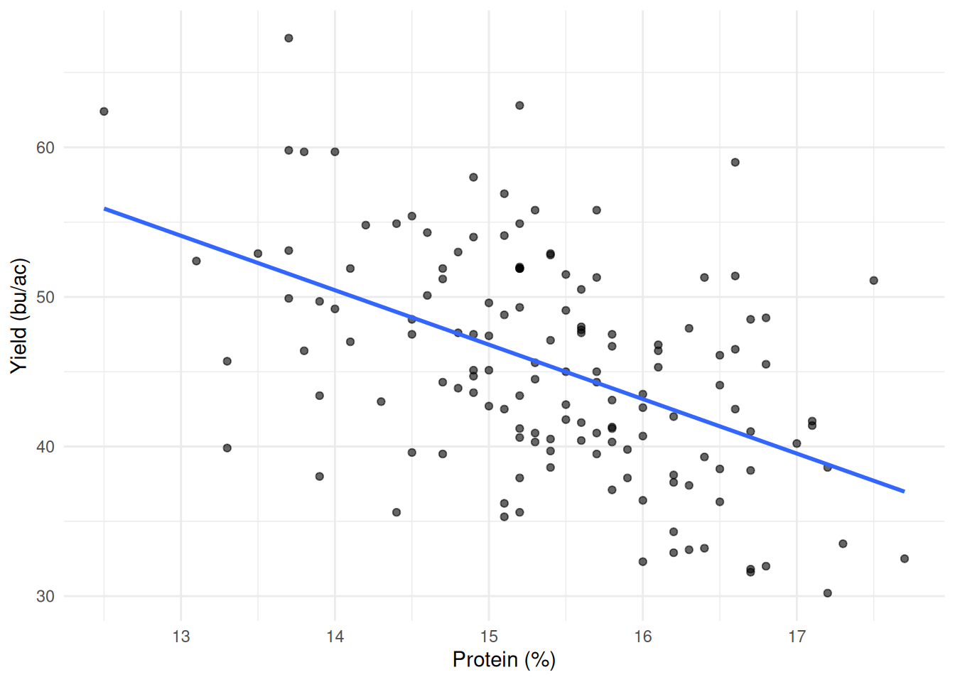
Step 2 – fit it and read the output.
protein_fit <- lm(yield_bu_ac ~ protein_pct, data = wheat_fields)

summary(protein_fit)
> protein_fit <- lm(yield_bu_ac ~ protein_pct, data = wheat_fields)
>
> summary(protein_fit)
Call:
lm(formula = yield_bu_ac ~ protein_pct, data = wheat_fields)
Residuals:
Min 1Q Median 3Q Max
-13.3920 -4.7184 -0.2008 4.9158 18.0154
Coefficients:
Estimate Std. Error t value Pr(>|t|)
(Intercept) 101.4037 8.4004 12.071 < 2e-16 ***
protein_pct -3.6397 0.5438 -6.693 4.77e-10 ***
---
Signif. codes: 0 '***' 0.001 '**' 0.01 '*' 0.05 '.' 0.1 ' ' 1
Residual standard error: 6.426 on 141 degrees of freedom
(3 observations deleted due to missingness)
Multiple R-squared: 0.2411, Adjusted R-squared: 0.2357
F-statistic: 44.8 on 1 and 141 DF, p-value: 4.773e-10
Step 3 – put the error in bushels.
c(MAE  = mean(abs(resid(protein_fit))),
  RMSE = sqrt(mean(resid(protein_fit)^2)))
> c(MAE = mean(abs(resid(protein_fit))),
+ RMSE = sqrt(mean(resid(protein_fit)^2)))
MAE RMSE
5.214471 6.381178 Step 4 – compare it with the baseline. The mean-only model had an RMSE of 7.31 bu/ac. Protein alone gets to 6.38, an improvement of about 13%. Real, but modest: most of what moves yield across these fields is still unaccounted for.
Step 5 – check the residuals.
ggplot(data.frame(fitted = fitted(protein_fit),
                  resid  = resid(protein_fit)),
       aes(x = fitted, y = resid)) +
  geom_point(alpha = 0.6) +
  geom_hline(yintercept = 0, linetype = "dashed") +
  labs(x = "Fitted value (bu/ac)", y = "Residual (bu/ac)") +
  theme_minimal()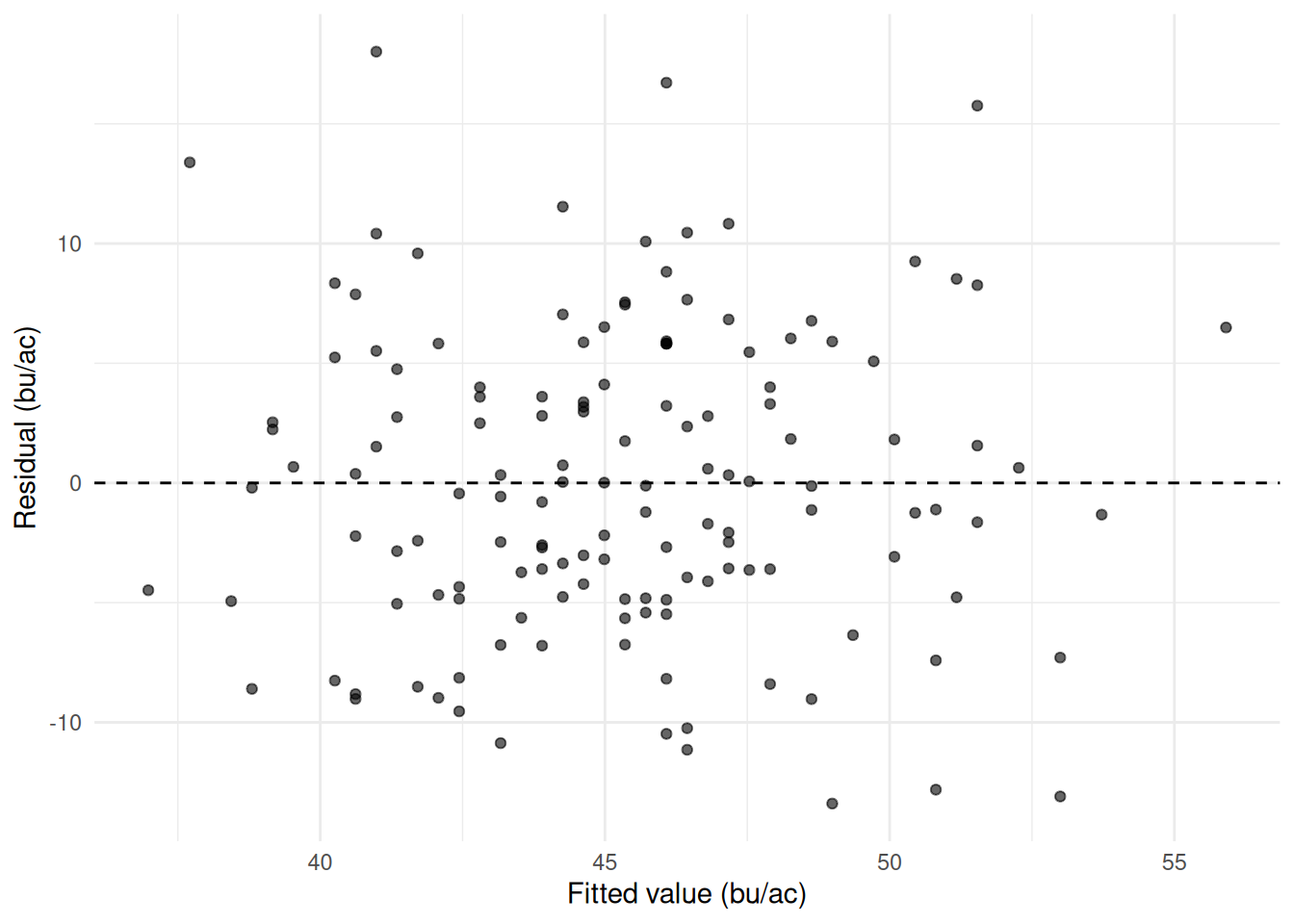
Step 6 – say what it does and does not show. Protein is negatively associated with yield – about 3.6 bu/ac for each extra percentage point – and knowing a field’s protein reduces prediction error by about an eighth against guessing the average. Note the three fields with no protein reading, which R drops silently: this model is fitted on 143 fields, not 146, and the error measures are not quite comparable with the earlier ones because of it. The slope is not a dilution effect that has been measured: soil zone drives both yield and protein, so this is a model with an obvious candidate for an omitted variable, and the sign table in Section 27.2 applies to it directly. Protein is also measured after harvest, which rules it out as a predictor for anyone who wants a forecast in June.