Up to this point, we have assumed a linear relationship between the explanatory and response variables. In a regression of yield on rainfall, this means 10 mm of rain in a dry year has the same effect as an additional 10 mm of rain in a wet year. That assumption is often wrong, and this chapter tries to give us the tools to correct that.
The trick is that we will still be estimating a “linear model”, in that there is a linear relationship between the variables in the model and the model’s coefficients. But the relationship between the explanatory and response variables will no longer be linear. Consider for example the following regression, which now has two components:
To fit this model, we give lm() two columns: rainfall and rainfall squared. It treats these as two explanatory variables, multiplying each by a coefficient and adding the results together. The coefficients enter in exactly the same way as in any other linear regression.
But when rainfall changes, both columns change together: rainfall squared grows faster as rainfall increases. This allows the effect of an additional millimetre of rain to vary with the amount of rainfall already received. The relationship between rainfall and yield can therefore be curved, even though the model is linear in its coefficients.
We will learn three options for functional forms – though there are many more: linear, logarithmic, and polynomial.
Throughout, log() means the natural logarithm (base e), which is what R gives you. The examples use the same two datasets as Section 24.8:
A linear response model is what we have been working with up to this point. It posits a linear relationship between the explanatory and response variables. In the example of yield and rainfall, this is not a great assumption. But it may be a closer approximation of the truth for other relationships, and it is a good starting point for any analysis.
25.2 Logarithms
Logging the explanatory variable
A common functional form is to take the logarithm of the explanatory variable. This means that instead of our regression being
To see how these models differ consider how a one unit change in x impacts both models. In the linear model, a one unit change in x changes y by \(\beta_1\) units. In the log model, a one unit change in x changes y by \(\beta_1 \times \log(x+1) - \beta_1 \times \log(x) = \beta_1 \times \log(\frac{x+1}{x})\). Evidently, as x gets larger, the fraction \(\frac{x+1}{x}\) gets smaller.
In this model, we can interpret \(\beta_1/100\) as approximately the change in y for a 1% change in x. All three percentage readings in this section are approximations – good for small changes, and drifting as the change gets larger, which we come back to at the end. As \(x\) gets larger, a 1% change in x is a larger absolute change, but the impact on y is the same. This is often called a diminishing returns model.
So consider the following regression of yield on fertilizer use, from the canola trial of Chapter 24:
# yield against the log of the nitrogen ratelog_fert <-lm(yield_bu_acre ~log(fertilizer_kg_ha), data = trial)coef(log_fert)summary(log_fert)$adj.r.squared
> # yield against the log of the nitrogen rate
> log_fert <- lm(yield_bu_acre ~ log(fertilizer_kg_ha), data = trial)
> coef(log_fert)
          (Intercept) log(fertilizer_kg_ha)
            -24.92900              16.26956
> summary(log_fert)$adj.r.squared
[1] 0.3335113
The coefficient is 16.27. Dividing by 100 gives the effect of a 1% increase in nitrogen: about 0.16 bu/ac. So going from 80 to 80.8 kg/ha buys 0.16 bu/ac, and so does going from 150 to 151.5 kg/ha – the same percentage, the same yield gain, even though the second case is nearly twice as much fertilizer.
Fitting the straight line to the same data gave a slope of 0.1315 bu/ac per kg/ha (Section 24.4), and an adjusted \(R^2\) of 0.3317 against 0.3335 here. The two forms fit this data about equally well (0.3335 against 0.3317). Similar fit does not tell us which shape is right; choosing between them needs an argument about how nitrogen response actually behaves, not a third decimal place.
Logging the response variable
We can also log the response variable. This means that instead of our regression being
We can interpret this in the inverse way that we interpreted the log of the explanatory variable: \(100 \times \beta_1\) now gives the percentage change in y that results from a one unit change in x.
Consider rainfall and canola yield across the RM data:
# the log of yield against rainfalllog_yield <-lm(log(Canola) ~ Precip_May_Aug_mm, data = canola)coef(log_yield)
> # the log of yield against rainfall
> log_yield <- lm(log(Canola) ~ Precip_May_Aug_mm, data = canola)
> coef(log_yield)
      (Intercept) Precip_May_Aug_mm
      3.097506495       0.001968345
The coefficient is 0.00197. Multiplying by 100 turns it into a percentage: the fitted model associates each additional millimetre of rain with about 0.2% more yield, so an extra 10 mm raises it by about 2%.
Notice what this form assumes. A 2% gain is a larger number of bushels on a good RM than on a poor one, so logging the response says the effect of rain is proportional to how much the field was going to yield anyway. That is a different claim from the linear model, which gives every RM the same 0.057 bu/ac per mm regardless of its starting point.
Logging both the explanatory and the response variable
The natural conclusion is that we could log both the explanatory and response variable. This gives the regression: \[
\log(y) = \beta_0 + \beta_1 \, \log(x) + \varepsilon
\]
Now the interpretation of \(\beta_1\) is the percentage change in y that results from a percentage change in x. You may already be familiar with this as the economic concept of an elasticity. For example, if \(\beta_1 = 0.5\), then a 10% increase in x would result in a 5% increase in y.
Taking rainfall and yield again, with both sides logged:
# both sides logged: the elasticity of yield with respect to rainfallelasticity <-lm(log(Canola) ~log(Precip_May_Aug_mm), data = canola)coef(elasticity)
> # both sides logged: the elasticity of yield with respect to rainfall
> elasticity <- lm(log(Canola) ~ log(Precip_May_Aug_mm), data = canola)
> coef(elasticity)
           (Intercept) log(Precip_May_Aug_mm)
             1.4706603              0.3867486
The elasticity is 0.387, so a 1% increase in rainfall goes with about a 0.39% increase in yield, and a 10% increase with about 3.9%.
One convenience of this form is that the elasticity is unit-free. It reads the same whether rainfall is recorded in millimetres or inches and whether yield is in bushels or tonnes, because both sides are percentages. Rescaling a logged variable only shifts the intercept, since \(\log(cx) = \log c + \log x\), so the coefficient is untouched.
Collecting the three in one place:
Form
Model
\(\beta_1\) reads as
log-x
\(y = \beta_0 + \beta_1 \log(x)\)
a 1% rise in x gives about \(\beta_1/100\) more y
log-y
\(\log(y) = \beta_0 + \beta_1 x\)
a 1-unit rise in x gives about \(100\beta_1\)% more y
log-log
\(\log(y) = \beta_0 + \beta_1 \log(x)\)
a 1% rise in x gives about \(\beta_1\)% more y
A caution on all three: the percentage readings are approximations, and they drift once the change is large. At 10% the approximation is close (3.87% against an exact 3.75%); at 50% it is noticeably off. For the elasticity the exact figure is \((1+\Delta)^{\beta_1} - 1\), which is where the 3.75% comes from: \(1.10^{0.387} - 1\). And log() is undefined at zero and below, so a column containing zeros cannot simply be logged.
25.3 Polynomials
A model of y on log(x) with a positive slope imposes diminishing marginal increases in y. Other log forms need not have this shape. Some relationships may instead rise and then fall. We might think of yields and rainfall as having such a relationship – at high levels of rain, additional precipitation would harm yields.
A potentially more flexible way of modelling this outcome is a quadratic model in which we have two explanatory variables: x and x squared. This gives us the regression: \[
\widehat{y} = \beta_0 + \beta_1 x + \beta_2 x^2
\]
If we recall our calculus, if we take the derivative of this equation with respect to x, we get: \[
\frac{d\widehat{y}}{dx} = \beta_1 + 2\beta_2 x
\]
This is the instantaneous slope at x. The exact change from \(x\) to \(x+1\) is \(\beta_1 + \beta_2(2x+1)\), which differs by \(\beta_2\) – small enough here that the table below uses the slope. This means that the effect of x on y is not constant, but depends on the value of x. If \(\beta_1\) is positive and \(\beta_2\) is negative, then the effect of x on y will be positive at low values of x, but will eventually become negative at high values of x.
Consider the relationship between rainfall and yields:
# rainfall and its squarerain_quad <-lm(Canola ~ Precip_May_Aug_mm +I(Precip_May_Aug_mm^2),data = canola)coef(rain_quad)summary(rain_quad)$adj.r.squared
> # rainfall and its square
> rain_quad <- lm(Canola ~ Precip_May_Aug_mm + I(Precip_May_Aug_mm^2),
+                 data = canola)
> coef(rain_quad)
           (Intercept)      Precip_May_Aug_mm I(Precip_May_Aug_mm^2)
         18.4530497328           0.1085906940          -0.0001135533
> summary(rain_quad)$adj.r.squared
[1] 0.17784
In R, I(x^2) adds the squared term. The I() is required: inside a formula ^ means something else, and I() says “treat this arithmetically”.
This is the case described above: \(\beta_1\) is positive (0.1086) and \(\beta_2\) is negative (-0.000114), so rain helps at low levels and helps less and less as the season gets wetter. Putting those into \(\beta_1 + 2\beta_2 x\) gives the effect of one more millimetre at any rainfall level:
May–August rainfall
Effect of 1 more mm
100 mm
0.086 bu/ac
200 mm
0.063 bu/ac
300 mm
0.041 bu/ac
400 mm
0.018 bu/ac
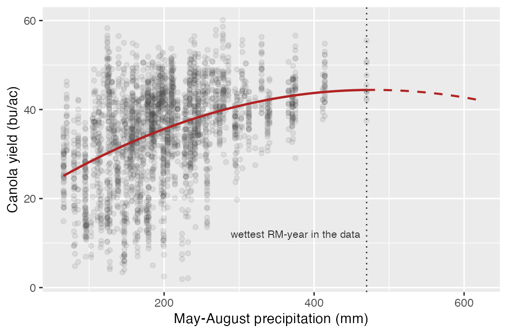
A millimetre of rain in a dry season is worth nearly five times a millimetre in a wet one. That is the thing the straight-line model could not say, and it is why neither coefficient can be read on its own – 0.1086 is not “the effect of rainfall”, it is the effect at zero rainfall, which no RM-year in this data comes close to.
Figure 25.1: Rainfall with a quadratic fitted. The dashed section is the model carried past the data.
The turning point
Setting \(\beta_1 + 2\beta_2 x = 0\) and solving gives the top of the curve, at \(-\beta_1 / (2\beta_2)\). Here that is 478 mm.
However, in our data the wettest year we observe is 470 mm. So we don’t have much confidence in predicting what happens after that. The dashed part of Figure 25.1 is the model carried past the data. That dashed section is a model prediction, but not one the data supports – it is the fitted shape carried into a range no RM-year reached.
In general, you should report this turning point only when it sits comfortably inside the data.
25.4 Choosing a Form
So how do we choose our functional form? The most important thing is to understand the process that you are modelling. For example, we should learn from the agronomic experts what the relationship between rainfall and yields should plausibly look like. A straight line may be a useful approximation over a limited range, even if the relationship curves over a wider range.
Second, we can look at the data. A scatter plot of the two variables can show us whether the relationship is linear or curved, and whether there are any outliers that might be affecting the relationship. However, keep in mind that there may be other variables that impact our data that are correlated with the explanatory variable.
Third, we can compare the fit of different models. We can compare the adjusted \(R^2\) of different models to see which one fits the data better. But we should treat this with some caution. Adding a term to a nested model fitted on the same rows cannot decrease the plain \(R^2\), so on that measure a polynomial will always beat a straight line. The adjusted \(R^2\) charges the model for each term it uses, so it can fall when the extra term buys nothing:
Model
\(R^2\)
Adjusted \(R^2\)
Linear
0.1708
0.1705
Log of rainfall
0.1760
0.1757
Quadratic
0.1784
0.1778
Cubic
0.1784
0.1776
The cubic matches the quadratic on \(R^2\) and does worse once the extra term is paid for: its small improvement in fit does not cover the penalty for the extra coefficient.
These four are comparable because they share the same response and the same rows. A model of log(Canola) cannot be put in this table – its \(R^2\) is a share of the variation in log yield, which is a different quantity.
But notice how little separates any of these. All four sit near 0.17, so fit alone is not telling us much – what separates them is the shape each one claims, and whether that shape is one an agronomist would recognise. The quadratic is a reasonable candidate because it allows the rainfall response to flatten. Its slightly better fit does not establish that it is the true relationship or the best model for prediction.