Field-level yield data become more useful when it is linked to other data sets. For example, combining yield records with information about management practices, wetlands, soil characteristics and weather allows us to model why some parts of a field yield more than others, and how those relationships vary across seasons. Farmers can use these datasets to understand their own fields, but the possibilities become greater when academic researchers, agribusiness companies or government agencies bring together data from many farms. They can compare practices across different soils and growing conditions, investigate whether patterns hold beyond an individual field, and develop models that help predict outcomes elsewhere.
In this chapter, we will illustrate this approach by merging our yield data with one other dataset: a satellite-derived vegetation index. Vegetation indices use the light reflected from the land surface to describe vegetation. We will use normalised difference vegetation index or NDVI, which measures the greenness of the crop canopy based on how different wavelengths of light are reflected off the crop. A more detailed explanation is here.
Because satellite images are available during the growing season, NDVI can help predict yields before harvest. Such forecasts can help farmers plan storage and marketing, agribusiness companies anticipate the volume of grain they will handle, and governments assess regional production and emerging shortfalls. Satellite observations also cover many fields repeatedly, making it possible to track crop development over a much larger area than could be visited on the ground. Here, we will start with a simpler question: how closely does the greenness of different parts of our field during the season relate to the yield measured at harvest?
We will use measures of NDVI stored in raster data – these data give the NDVI value for 10m by 10m pixels on the field in different weeks of the growing season. The data come from the Sentinel-2, a European space agency satellite that provides high-resolution images of the Earth’s surface. As we will see, early in the season NDVI is a poor predictor of yield, because the crop has not developed yet. Late in the season it is also a poor predictor of yield, as the crop is senescing or already harvested. The sweet spot is in the middle of the season, when the crop is flowering and filling pods.
The data is in this zip file: ndvi_raster.zip. Unzip it into your data/ folder and you will have eight rasters, each a 10 m image of the field at one point in the 2026 growing season.
Week
Dates
File
Crop stage
25
15-21 June
kernen_b1_ndvi_2026-W25.tif
canopy coming up
26
22-28 June
Not available (cloudy)
canopy coming up
27
29 June - 5 July
Not available (cloudy)
canopy closing
28
6-12 July
kernen_b1_ndvi_2026-W28.tif
canopy closed
29
13-19 July
Not available (cloudy)
flowering
30
20-26 July
kernen_b1_ndvi_2026-W30.tif
flowering
31
27 July - 2 August
kernen_b1_ndvi_2026-W31.tif
pod fill
32
3-9 August
kernen_b1_ndvi_2026-W32.tif
pod fill
33
10-16 August
Not available (cloudy)
pod fill
34
17-23 August
kernen_b1_ndvi_2026-W34.tif
starting to turn
35
24-30 August
Not available (cloudy)
starting to turn
36
31 August - 6 September
kernen_b1_ndvi_2026-W36.tif
senescing
37
7-13 September
kernen_b1_ndvi_2026-W37.tif
ripe or swathed
Note that five of the weeks are missing, because it was cloudy when the satellite passed over the field.
32.1 Reading in the satellite data
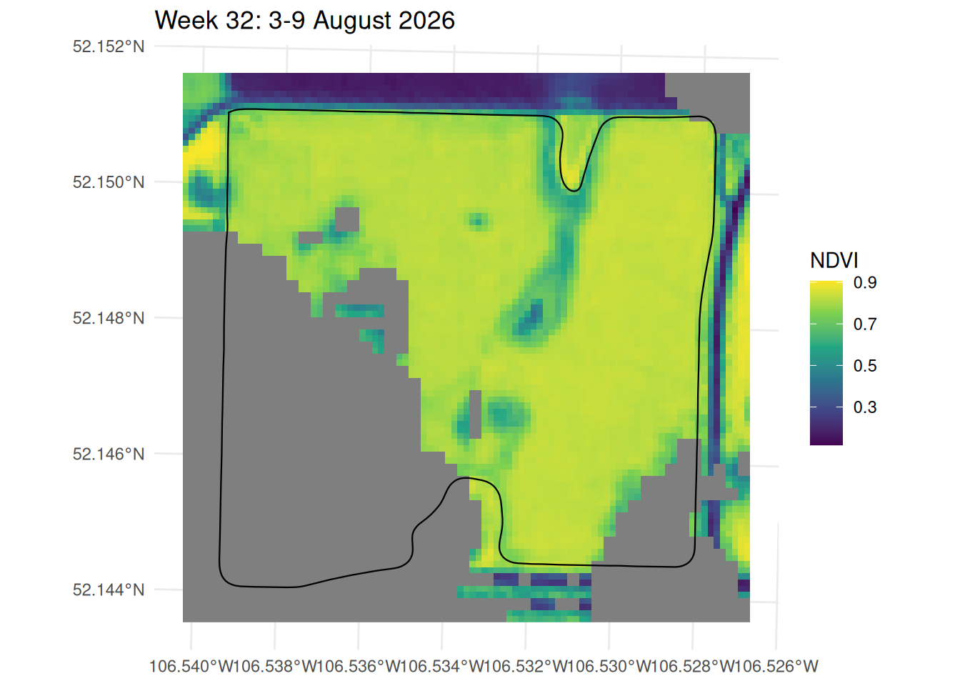
Let’s start by reading in one week of the NDVI data and plotting it on our field, without matching it to the yield data yet. The NDVI values are stored in a raster, which from Chapter 21 we know we can read with the terra package and plot with tidyterra. I am going to read in and plot the week 32 data. I am also appending the border of the field to the plot, so we can see where the pixels sit relative to the field boundary.
> library(terra)
terra 1.9.50

Attaching package: 'terra'
The following object is masked from 'package:tidyr':

    extract
> library(sf)
> library(tidyterra)

Attaching package: 'tidyterra'
The following object is masked from 'package:stats':

    filter
> library(exactextractr)
>
> ##Read in week 32
> wk_32 <- rast("data/ndvi_raster/kernen_b1_ndvi_2026-W32.tif")
>
> boundary <- st_read("data/kernen_b1_boundary.geojson", quiet = TRUE)
>
> ggplot() +
+   geom_spatraster(data = wk_32) +
+   geom_sf(data = boundary, fill = NA, colour = "black", linewidth = 0.4) +
+   scale_fill_viridis_c(name = "NDVI") +
+   labs(title = "Week 32: 3-9 August 2026") +
+   theme_minimal()
In the map lighter colours are higher vegetation. Cells in grey are NA – these were masked as cloud or cloud shadow, and here they are a single shadow lying across the southwest third of the field. Set against the yield map from Chapter 31 this roughly matches: the dark patches sit in the wetlands or outside the field boundary, and inside the boundary the crop reads a fairly uniform 0.7 to 0.8.
32.2 Merging satellite and yield data
The two layers do not share a key. The yield is a table of readings with coordinates; the NDVI is a raster of 10 m pixels. Joining them means putting both on the same grid, and the simplest way to do that is to pick one grid and move the other onto it.
The satellite’s grid is the one to pick, because it is fixed. We can put the yield readings anywhere we like, but we cannot move the pixels.
rasterize() does the moving. It is the reverse of extract(): instead of reading a raster at a set of points, it takes points and returns a raster, with fun saying how to combine the points that land in the same cell. Giving it wk_32 as the template is what makes the two line up – the yield raster comes out with the same extent, resolution and origin as the satellite image.
That matters more than it sounds. Two rasters at the same resolution are not necessarily on the same grid. Had we built a 20 m yield grid of our own starting at easting 394,660, and the satellite’s cells started at 394,605, every yield cell would straddle two NDVI cells and any join between them would be approximate. Building one raster from the other removes the problem instead of correcting for it.
harvest <-read_csv("output/kernen_b1_per_second.csv", show_col_types =FALSE) |>filter(!flag_any)##The readings as points, projected to match the rasterharvest_sf <- harvest |>st_as_sf(coords =c("longitude", "latitude"), crs =4326) |>st_transform(32613) |>vect()##Mean yield of the readings falling in each cell, on the NDVI gridyield <-rasterize(harvest_sf, wk_32, field ="yield", fun = mean)yield
> harvest <- read_csv("output/kernen_b1_per_second.csv", show_col_types = FALSE) |>
+   filter(!flag_any)
>
> ##The readings as points, projected to match the raster
> harvest_sf <- harvest |>
+   st_as_sf(coords = c("longitude", "latitude"), crs = 4326) |>
+   st_transform(32613) |>
+   vect()
>
> ##Mean yield of the readings falling in each cell, on the NDVI grid
> yield <- rasterize(harvest_sf, wk_32, field = "yield", fun = mean)
>
> yield
class       : SpatRaster
size        : 90, 93, 1  (nrow, ncol, nlyr)
resolution  : 10, 10  (x, y)
extent      : 394605, 395535, 5778120, 5779020  (xmin, xmax, ymin, ymax)
coord. ref. : WGS 84 / UTM zone 13N (EPSG:32613)
source(s)   : memory
varname     : kernen_b1_ndvi_2026-W32
name        :   mean
min value   : 11.166
max value   : 56.116
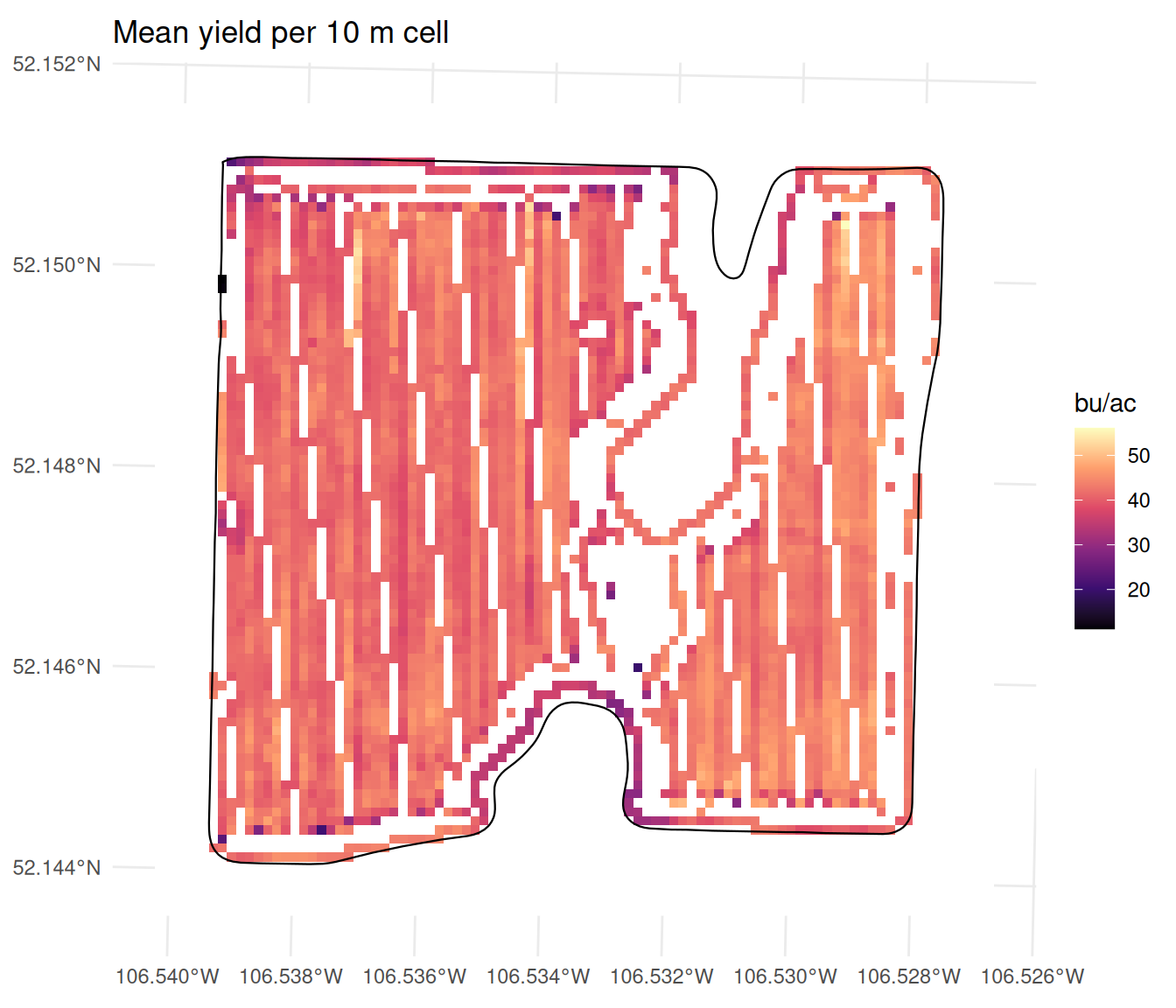
Figure 32.1: Mean yield in each 10 m cell of the satellite’s grid. The stripes are the combine’s passes; cells between them never got a reading.
Figure 32.2: Mean yield in each 10 m cell of the satellite’s grid. The stripes are the combine’s passes; cells between them never got a reading.
The striping is the combine. A satellite sees the whole field at once, but a combine only measures the ground it drives over, and at 10 m the cells are finer than the spacing between pass centres, so whole columns of cells fall between passes and stay empty. 3,648 of the 8,370 cells get a yield. That is worth remembering when we come to compare the two layers: the NDVI is missing where cloud fell, the yield is missing where the combine did not go, and those are different parts of the field.
32.3 Correlating the two rasters
We can get the correlation between yield and week 32 NDVI by simply using the cor() argument that we learned in Section 23.1. Note that we need to use values() to get the values out of the raster.
##values() returns a one-column matrix, so as.numeric() gives a plain numbercor(values(wk_32), values(yield), use ="complete.obs") |>as.numeric()
> ##values() returns a one-column matrix, so as.numeric() gives a plain number
> cor(values(wk_32), values(yield), use = "complete.obs") |> as.numeric()
[1] 0.2606881
The correlation between week 32 NDVI and yield is 0.261, which is a moderate positive correlation. Recall that an NDVI is only a measure of how green the crop is at one particular moment – our end of harvest yield is the result of weather conditions and management decisions that occur after week 32. Moreover, the NDVI is only a measure of the top of the canopy, and does not tell us about the number of pods or seeds that are developing below. So it is not surprising that the correlation is not higher.
Given we have many weeks of data, we might be interested in seeing how the correlation changes over the season. We can read in all the weeks and stack them into one object, and then use cor() to get the correlation between yield and each week of NDVI.
##Read each weekwk_25 <-rast("data/ndvi_raster/kernen_b1_ndvi_2026-W25.tif")wk_28 <-rast("data/ndvi_raster/kernen_b1_ndvi_2026-W28.tif")wk_30 <-rast("data/ndvi_raster/kernen_b1_ndvi_2026-W30.tif")wk_31 <-rast("data/ndvi_raster/kernen_b1_ndvi_2026-W31.tif")wk_34 <-rast("data/ndvi_raster/kernen_b1_ndvi_2026-W34.tif")wk_36 <-rast("data/ndvi_raster/kernen_b1_ndvi_2026-W36.tif")wk_37 <-rast("data/ndvi_raster/kernen_b1_ndvi_2026-W37.tif")##Stack them into one object, one layer per weekall_weeks <-c(yield, wk_25, wk_28, wk_30, wk_31, wk_32, wk_34, wk_36, wk_37)names(all_weeks) <-c("yield", "W25", "W28", "W30", "W31", "W32", "W34", "W36", "W37")##Get the correlation between yield and each week of NDVIcor(values(all_weeks), use ="pairwise.complete.obs")
The correlation table that is printed out give the correlation between yield and each week of NDVI in the first row and the first column (note that the first row and the first column are exactly the same, as are all other row and column pairs). We can see a positive correlation between yield and NDVI in weeks 28-34, which is when the crop is flowering and filling pods. In other weeks, the correlation is actually negative – we would have expected this relationship to be weak, as the crop is either not yet developed or has already senesced or been harvested.
We should also note that the correlation between the weeks in the middle of the season is very high – weeks 28 to 32 all have correlations above 0.9. This is also expected – cells that are green in one week, are quite likely to be green in the next.
32.4 Prediction with a linear model
Suppose now that we wanted to be able to predict what yields would be if we grew canola on the same field in a different year. To do this, we could run a linear model with the yield as the response and the NDVI values from the different weeks as the predictors.
I should caution that this is not a good way to build a yield prediction model. The problem is not the number of observations – we have thousands of cells. It is that every one of them comes from the same field in the same year, under one soil, one variety and one season’s weather. The model can learn how greenness and yield vary from one end of B-1 to the other in 2026, and that is all it can learn. Nothing in the data says what happens in a dry year, on a different soil, or in a field that averages 30 bushels instead of 42. So please treat this section as an illustration of the process rather than a practical tool.
As we learned in Chapter 28, we should hold back some of the data to test the model on. We will hold back a random 30% of the cells, and fit the model on the remaining 70%. We can do this by using the sample() function to select a random set of rows to hold back. We can partition our data into a training set and a test set, and then fit the model on the training set and evaluate it on the test set.
##Set a seed -- this will make the random draw repeatable, so you get the same training and test sets each time you run this codeset.seed(123)## Convert the raster stack to a data frame, with one row per cell and one column per week.## Most cells carry an NA somewhere -- the combine never covered them, or cloud hid them that## week -- and those rows stay in. lm() drops them when it fits, so the model uses fewer rows## than the counts printed belowdata <-as.data.frame(all_weeks) ##Hold back a random 30% to test on. set.seed() makes the draw repeatabletest_rows <-sample(nrow(data), nrow(data) *0.3)train_data <- data[-test_rows, ]test_data <- data[test_rows, ]c(train =nrow(train_data), test =nrow(test_data))
> ##Set a seed -- this will make the random draw repeatable, so you get the same training and test sets each time you run this code
> set.seed(123)
>
> ## Convert the raster stack to a data frame, with one row per cell and one column per week.
> ## Most cells carry an NA somewhere -- the combine never covered them, or cloud hid them that
> ## week -- and those rows stay in. lm() drops them when it fits, so the model uses fewer rows
> ## than the counts printed below
> data <- as.data.frame(all_weeks)
>
> ##Hold back a random 30% to test on. set.seed() makes the draw repeatable
> test_rows <- sample(nrow(data), nrow(data) * 0.3)
>
> train_data <- data[-test_rows, ]
> test_data  <- data[test_rows, ]
>
> c(train = nrow(train_data), test = nrow(test_data))
train  test
 5859  2511
We can start just using one week as a predictor. Week 28 has the strongest correlation with yield, at 0.445, so let’s use that as our predictor. We can fit a linear model with lm() and then look at the summary of the model to see how well it fits the data.
## Fit a linear model with yield as the response and week 28 as the predictorone_week <-lm(yield ~ W28, data = train_data)summary(one_week)
> ## Fit a linear model with yield as the response and week 28 as the predictor
> one_week <- lm(yield ~ W28, data = train_data)
>
> summary(one_week)

Call:
lm(formula = yield ~ W28, data = train_data)

Residuals:
     Min       1Q   Median       3Q      Max
-20.8981  -1.7433  -0.1163   1.9045  11.2318

Coefficients:
            Estimate Std. Error t value Pr(>|t|)
(Intercept)    4.943      1.375   3.595  0.00033 ***
W28           43.321      1.607  26.964  < 2e-16 ***
---
Signif. codes:  0 '***' 0.001 '**' 0.01 '*' 0.05 '.' 0.1 ' ' 1

Residual standard error: 2.857 on 2541 degrees of freedom
  (3316 observations deleted due to missingness)
Multiple R-squared:  0.2225,	Adjusted R-squared:  0.2222
F-statistic: 727.1 on 1 and 2541 DF,  p-value: < 2.2e-16
Greenness in the second week of July explains about 22% of the variation in yield between cells, and the coefficient says that one tenth of an NDVI point greener yielded roughly 4 bu/ac more.
To see how well the model predicts both in sample and out of sample, let’s use the RMSE we learned in Section 28.3. We can calculate this both for the training data (in sample) and the test data (out of sample).
The RMSE is 2.86 bu/ac in-sample and 2.95 out of sample. To get a sense of how good this is, we can compare it to the standard deviation of the yield itself – the standard deviation is essentially the RMSE we would get if we just guessed the mean yield to predict for every cell. The standard deviation of the yield is 3.22 bu/ac, so knowing the NDVI takes the typical error from 3.22 down to 2.95 - which is a modest improvement.
Now let us add more weeks. Week 28, week 30 and week 31 all fall in the part of the season when the satellite is looking at a closed canopy. Weeks 32 and 34 correlate about as strongly, but both are cut into by cloud, so adding them would cost us a third of the rows – we leave them out for now.
three_weeks <-lm(yield ~ W28 + W30 + W31, data = train_data)summary(three_weeks)##In sample predictioninsample_prediction_3w <-predict(three_weeks, train_data)##In sample RMSEsqrt(mean((train_data$yield-insample_prediction_3w)^2, na.rm =TRUE))##Out of sample predictionoutsample_prediction_3w <-predict(three_weeks, test_data)##Out of sample rmsesqrt(mean((test_data$yield-outsample_prediction_3w)^2, na.rm =TRUE))
Three images instead of one moves the out-of-sample error from 2.95 to 2.89 bu/ac – which is, again a very small improvement. There is something odd in that output. The coefficient on week 30 NDVI is negative. Taken literally this means that a higher NDVI in week 30 is associated with a lower yield. This is counterintuitive, as we would expect a higher NDVI to indicate better crop health and thus higher yields. The issue is that the NDVI readings across our three weeks are highly correlated with each other. This multicollinearity can lead to unstable coefficients.
This is worth setting beside the caution above. The out-of-sample test tells us the model predicts held-out cells of B-1 in 2026 about as well as it predicts the cells it was fitted on, and that is a genuine result. It says nothing about how the model would do on a field it has never seen, because no field it has never seen appears anywhere in the data. Thousands of cells cannot supply a variety the data does not contain.