29  Field-level data

Farms now generate large amounts of field-level data: combines record yield, seeders and sprayers record what they apply, and satellites and drones measure vegetation through the growing season. Platforms such as John Deere Operations Center, FieldView and PCT Agcloud provide tools for organising, mapping and analysing these records.

However, learning to work with the data yourself lets you analyze a range of questions unconstrained by those that are supported by a particular platform. It also lets you combine data from different sources, and to check the quality of the data before you trust it. These skills are useful on an individual farm, in an agribusiness company pooling data from different customers to compare patterns across farms, or in agronomic research combining field observations with experimental results. In this module, we will learn to read and clean combine data, create yield maps, and combine yield data with satellite data for simple modelling.

In this chapter, I will introduce the dataset that we will work with – combine harvester data from a University of Saskatchewan research field. I will also discuss how the data are produced, and some of the issues that arise when working with them. The next three chapters will then work through the data cleaning, mapping and modelling.

29.1 Field-level combine data

The file used in the next three chapters is from a canola field at the University of Saskatchewan’s Kernen farm, east of Saskatoon. The data was downloaded from John Deere Operations Center as a shapefile and converted to a CSV, which is the form you will open it in. It is 1,639,804 rows long, and has fourteen columns. Each row in the data gives:

1. The location of each section of the combine header each second, in longitude and latitude.
2. The yield, moisture and ground speed measured by the combine’s sensors.
3. Other details about the field (such as elevation) and the crop (such as variety)

The complete list of columns in the data are in the table below:

Column	Description
longitude, latitude	position of the centre of the section
Elevation	height, in feet
Heading	direction of travel, in degrees
IsoTime	timestamp, UTC
DISTANCE	travel since the last reading, in feet
VEHICLSPEED	ground speed, mi/hr
WetMass	wet grain mass per area, lb/ac
Moisture	grain moisture, %
SWATHWIDTH	width of the section, in feet
VARIETY	what was planted
SECTIONID	which strip of the header
VRYIELDVOL	yield, bu/ac, calculated from WetMass
DRYMATTER	dry matter, %, which is 100 - Moisture

Below are a set of rows from the data. The first three rows below (3,710-3,712) are three consecutive rows taken from when the combine has started actually harvesting (the first few rows of the data can have issues with measuring moisture and yield – see section Section 29.3). The next rows are randomly taken from throughout the file.

row	longitude	latitude	DISTANCE	SWATHWIDTH	VRYIELDVOL	SECTIONID	WetMass	Moisture	Heading	VARIETY	Elevation	IsoTime	VEHICLSPEED	DRYMATTER
3,710	-106.5393244	52.1505499	3.457	0.4987	40.40	7849	2101.1	7.5	179.91	340LL 2026	1694.00	2026-09-29T16:15:20.725Z	2.3543	92.5
3,711	-106.5393222	52.1505500	3.457	0.4987	40.40	7848	2101.1	7.5	179.91	340LL 2026	1694.00	2026-09-29T16:15:20.725Z	2.3543	92.5
3,712	-106.5393200	52.1505500	3.457	0.4987	40.40	7847	2101.1	7.5	179.91	340LL 2026	1694.00	2026-09-29T16:15:20.725Z	2.3543	92.5
407,747	-106.5284364	52.1478933	5.692	0.4987	42.58	7822	2214.5	6.3	357.93	340LL 2026	1705.94	2026-09-29T18:12:54.920Z	3.8900	93.7
408,041	-106.5284994	52.1479563	5.679	0.4987	41.79	7793	2173.5	6.3	0.88	340LL 2026	1705.66	2026-09-29T18:12:58.926Z	3.8873	93.7
411,194	-106.5283175	52.1486021	5.628	0.4987	42.15	7843	2192.0	6.3	7.27	340LL 2026	1703.98	2026-09-29T18:13:40.920Z	3.8341	93.7
1,217,347	-106.5359123	52.1503374	5.338	0.4987	44.05	7862	2291.0	6.0	360.00	340LL 2026	1699.48	2026-09-29T23:21:35.065Z	3.6296	94.0
1,218,234	-106.5360683	52.1505001	5.538	0.4987	45.22	7792	2351.9	5.8	359.89	340LL 2026	1699.33	2026-09-29T23:21:46.065Z	3.7849	94.2

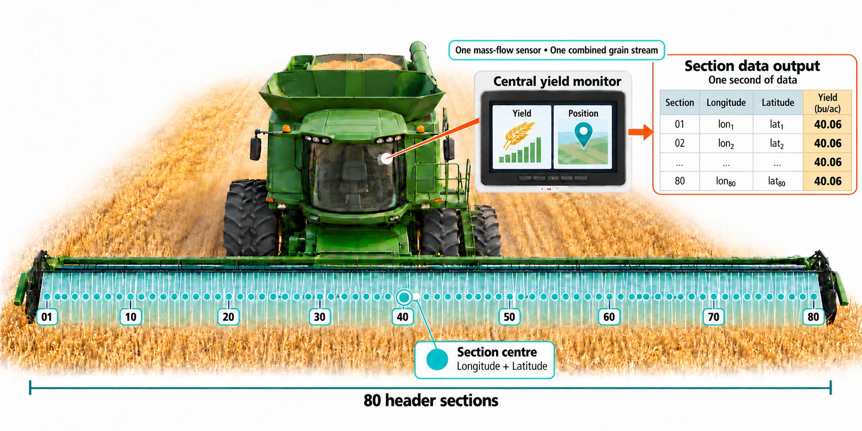
Let’s first notice that the first three rows in the table above are almost identical except for the longitude, latitude and SECTIONID. This is because yield and moisture are measured by sensors reading the whole grain stream, and speed by a single sensor on the machine, while the longitude and latitude capture the position of each section of the header. The following picture illustrates this: the combine’s header is divided into eighty sections and the display usually records one row for each section that is cutting, but the yield measurements all come from a central yield monitor. A handful of timestamps break that pattern and carry a single row for the whole header instead, so it is safer to think of the file as one row per section most of the time rather than always.

Figure 29.1: One second of harvesting, as the file records it. Each section is about six inches of the forty-foot header, and each gets its own row with its own longitude and latitude. The yield is the same on all of them, because it comes from one sensor measuring one grain stream.

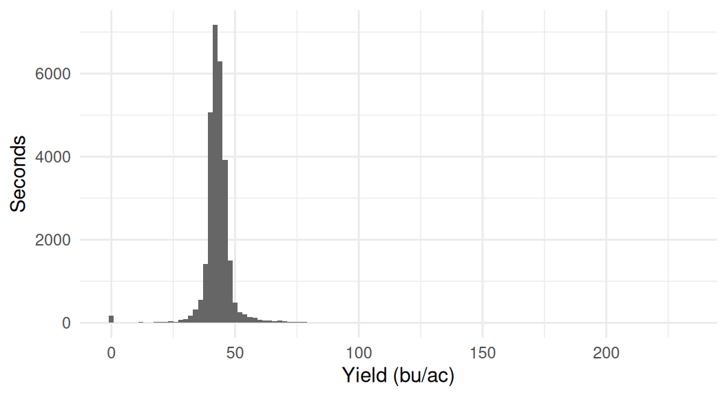
Of course, the most important part of the data is yield. The monitor divides the wet mass of grain that passed through the sensor in that second by the area of ground cut in that second, which gives WetMass in pounds per acre. Turning that into bushels per acre needs one more step: dividing by the weight of a bushel of the crop. In this file WetMass is 52.01 times VRYIELDVOL on almost every row, which is that conversion for canola. Below we plot a histogram of the yield values in the file in each second. The monitor also records the moisture of the grain using a moisture sensor.

── Attaching core tidyverse packages ──────────────────────── tidyverse 2.0.0 ──
✔ dplyr     1.2.1     ✔ readr     2.2.0
✔ forcats   1.0.1     ✔ stringr   1.6.0
✔ ggplot2   4.0.3     ✔ tibble    3.3.1
✔ lubridate 1.9.5     ✔ tidyr     1.3.2
✔ purrr     1.2.2     
── Conflicts ────────────────────────────────────────── tidyverse_conflicts() ──
✖ dplyr::filter() masks stats::filter()
✖ dplyr::lag()    masks stats::lag()
ℹ Use the conflicted package (<http://conflicted.r-lib.org/>) to force all conflicts to become errors

Attaching package: 'arrow'


The following object is masked from 'package:lubridate':

    duration


The following object is masked from 'package:utils':

    timestamp

Figure 29.2: Reported yield for each second of harvesting. Twenty-four seconds reading above 250 bu/ac are left off the plot so the rest of the distribution is visible.

Most seconds report something in the low forties, which is a sensible canola yield, and the distribution is tight. But we can note there are several zero yields, which would capture times when the combine was running but not cutting any crop, and a handful of very high yields that are likely errors in the data.

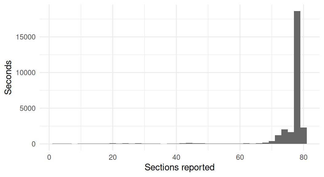
Note that not every section is active every second. The header is forty feet wide, and the combine may be cutting a swath that is narrower than that, in this case some sections will be missing from the data. In the following graph we show a histogram of the number of sections reported each second.

Figure 29.3: How many of the eighty sections reported in each second. Full width is the common case, but a quarter of the seconds are part-width passes.

Nearly three quarters of the seconds are at or near full width. The rest are spread thinly across every count down to one, and those are the passes along the field edge and around sloughs, where only part of the header was in standing crop.

29.1.1 Alternative file formats

Different machines will produce data in different formats. The file we are working with is an export from John Deere Operations Center, but other manufacturers have their own proprietary formats. Some ways in which this data can differ:

What a row represents. In our data, a row gives the location of one section of the header in one second, and the yield is the same on all of them. Other exports give one row per second, with the position at the centre of the header.

How often it logs. Every second is common but it can vary. Logging on a clock means the spacing on the ground depends on speed: this combine averaged 3.7 mph, a reading every 1.6 metres, but only 0.9 metres where it slowed to 2 mph. Some monitors log by distance instead, which evens out the spacing on the ground and lets the time between readings vary.

Which columns exist. Expect position, a flow or mass measurement, and some version of yield, though not always in bu/acre. There may be additional columns, such as the number of passes made across the field, which would allow you to isolate one pass at a time.

The names of the columns. VRYIELDVOL, WetMass and SWATHWIDTH are Deere’s names for yield, flow and header width.

All this is to say that the specifics of any one file are less important than understanding the general structure and behaviour of the data.

29.2 Other types of field-level data

Harvest produces the most data, but it is not the only operation that produces data. Planters log seeding rate, seed spacing and down-force. Sprayers log the rate applied, the boom sections that were on, the speed and often the nozzle pressure. Fertiliser spreaders and air carts log rate by product and by bin, and tillage equipment logs depth and position. All of this is as-applied data, and like yield data it records what a machine’s sensors reported, not what reached the soil.

Ideally, all this data is combined and can be analyzed. If seeding rate varied, you can match data from the seeder with the yield data to see how it affected the crop. If a sprayer missed a section, you can see whether that patch of crop suffered. If a fertilizer spreader applied more in one corner, you can see whether that corner yielded more.

29.3 Common issues with field-level data

There are a number of issues in working with field-level data that we need to understand before analyzing it.

Timing lag. Grain takes time to travel from the header to the sensor, so a reading is logged some distance after the ground it came from. A monitor may correct for this with an assumed delay, and nothing in this export says whether it did or what delay it used. The true delay varies with speed, the type of crop and other issues, so we shouldn’t have 100% confidence in the location of a yield reading.

Calibration. The machine operator needs to calibrate the yield monitor by weighing a few loads on a scale and entering the true weights. Miscalibration can shift yields on an entire field.

Reliability varies throughout the field, and is worst at the edges. Once the combine is running in straight lines the flow of grain through the monitor becomes fairly even. But at the edges of the field, it can be more variable. Together with issues of timing lag, this can make the noise in the data greater around the edges of the field.

Noise in GPS data. Longitude and latitude come from a receiver on the cab roof, and how close they are to the truth varies with the satellites overhead, obstructions such as a shelterbelt, and the atmosphere.

Moisture readings are unreliable at the edges. The chamber needs grain in it to read, so readings early in a session can be low before it fills.