30  Working with Real Machinery Data

In this chapter, we are going to read in combine data from a canola field at the University of Saskatchewan’s Kernen farm, east of Saskatoon. The data was downloaded from John Deere Operations Center as a shapefile and converted to a CSV and a parquet file.

You can download the file in one of two formats:

  1. A CSV file: kernen_b1_raw_full.csv.zip, which is 13 MB zipped and 241 MB once you unzip it.

  2. A parquet file: kernen_b1_raw_full.parquet, which is 9.5 MB and holds exactly the same data. Parquet files store the data much more compactly, and you can read them in using the function read_parquet() from the arrow package.

Both options give you the same data frame, so use whichever you prefer.

30.1 Importing machinery data

In the code below I read in the parquet file using read_parquet() from the arrow package, and the csv file using read_csv() – both give the same data. clean_names() is from the janitor package, and puts the column names into a consistent lower-case style so we are not switching between VRYIELDVOL and IsoTime as we work.

library(tidyverse)
library(arrow)
library(janitor)

##Read in parquet file and summarize yield data
harvest <- read_parquet("data/kernen_b1_raw_full.parquet") |>
  clean_names()

summary(harvest$vryieldvol)
dim(harvest)

##The csv arrives zipped, so unzip it before reading
unzip("data/kernen_b1_raw_full.csv.zip", exdir = "data")

##Read in csv file and summarize yield data
harvest <- read_csv("data/kernen_b1_raw_full.csv", show_col_types = FALSE) |>
  clean_names()

summary(harvest$vryieldvol)
dim(harvest)
> library(tidyverse)
> library(arrow)

Attaching package: 'arrow'
The following object is masked from 'package:lubridate':

    duration
The following object is masked from 'package:utils':

    timestamp
> library(janitor)

Attaching package: 'janitor'
The following objects are masked from 'package:stats':

    chisq.test, fisher.test
> 
> ##Read in parquet file and summarize yield data
> harvest <- read_parquet("data/kernen_b1_raw_full.parquet") |>
+   clean_names()
> 
> summary(harvest$vryieldvol)
    Min.  1st Qu.   Median     Mean  3rd Qu.     Max. 
    0.00    40.65    42.58    43.31    44.71 20096.68 
> dim(harvest)
[1] 1639804      14
> 
> ##The csv arrives zipped, so unzip it before reading
> unzip("data/kernen_b1_raw_full.csv.zip", exdir = "data")
> 
> ##Read in csv file and summarize yield data
> harvest <- read_csv("data/kernen_b1_raw_full.csv", show_col_types = FALSE) |>
+   clean_names()
> 
> summary(harvest$vryieldvol)
    Min.  1st Qu.   Median     Mean  3rd Qu.     Max. 
    0.00    40.65    42.58    43.31    44.71 20096.68 
> dim(harvest)
[1] 1639804      14

We can also look at the structure of the data frame using glimpse(), which shows the column names, types, and a preview of the data. It is also a good idea to look at the data in the data viewer within Positron.

glimpse(harvest)
> glimpse(harvest)
Rows: 1,639,804
Columns: 14
$ longitude   <dbl> -106.5394, -106.5394, -106.5393, -106.5393, -106.5393, -10…
$ latitude    <dbl> 52.15104, 52.15104, 52.15102, 52.15102, 52.15102, 52.15102…
$ distance    <dbl> 0.700, 2.037, 0.654, 0.654, 0.654, 0.654, 0.654, 0.654, 0.…
$ swathwidth  <dbl> 2.9921, 7.9790, 0.4987, 0.4987, 0.4987, 0.4987, 0.4987, 0.…
$ vryieldvol  <dbl> 0, 0, 0, 0, 0, 0, 0, 0, 0, 0, 0, 0, 0, 0, 0, 0, 0, 0, 0, 0…
$ sectionid   <dbl> 7823, 7823, 7816, 7817, 7818, 7819, 7820, 7821, 7822, 7823…
$ wet_mass    <dbl> 0, 0, 0, 0, 0, 0, 0, 0, 0, 0, 0, 0, 0, 0, 0, 0, 0, 0, 0, 0…
$ moisture    <dbl> 0, 0, 0, 0, 0, 0, 0, 0, 0, 0, 0, 0, 0, 0, 0, 0, 0, 0, 0, 0…
$ heading     <dbl> 111.61, 114.41, 120.98, 120.98, 120.98, 120.98, 120.98, 12…
$ variety     <chr> "---", "---", "340LL 2026", "340LL 2026", "340LL 2026", "3…
$ elevation   <dbl> 1694.34, 1694.26, 1694.34, 1694.34, 1694.34, 1694.34, 1694…
$ iso_time    <dttm> 2026-09-29 16:14:28, 2026-09-29 16:14:29, 2026-09-29 16:1…
$ vehiclspeed <dbl> 2.3596, 2.3596, 2.1829, 2.1829, 2.1829, 2.1829, 2.1829, 2.…
$ drymatter   <dbl> 100, 100, 100, 100, 100, 100, 100, 100, 100, 100, 100, 100…
30.2 Aggregating the section headers to one row

Our first issue is that the file has one row per section of the header – and each section carries the same yield reading. To make this clear, let’s look at the time stamp “2026-09-29T16:15:20.725Z” – this is the 29th of September, 2026 at 16:15:20 (4:15 PM) and 725 milliseconds. We can see that there are 79 rows in this second, and the yield is the same for all of them. The only thing that differs is the section ID and the longitude and latitude of that section.

# Every row sharing one timestamp
one_second <- filter(harvest, iso_time == ymd_hms("2026-09-29T16:15:20.725Z"))

##Get number of rows for that second
nrow(one_second)

##Summarize the yield for that second
summary(one_second$vryieldvol)

##Show the sectionid
select(one_second, longitude, latitude, sectionid, moisture, elevation, vryieldvol) |>
  head(6)
> # Every row sharing one timestamp
> one_second <- filter(harvest, iso_time == ymd_hms("2026-09-29T16:15:20.725Z"))
> 
> ##Get number of rows for that second
> nrow(one_second)
[1] 79
> 
> ##Summarize the yield for that second
> summary(one_second$vryieldvol)
   Min. 1st Qu.  Median    Mean 3rd Qu.    Max. 
   40.4    40.4    40.4    40.4    40.4    40.4 
> 
> ##Show the sectionid
> select(one_second, longitude, latitude, sectionid, moisture, elevation, vryieldvol) |>
+   head(6)
# A tibble: 6 × 6
  longitude latitude sectionid moisture elevation vryieldvol
      <dbl>    <dbl>     <dbl>    <dbl>     <dbl>      <dbl>
1     -107.     52.2      7849      7.5      1694       40.4
2     -107.     52.2      7848      7.5      1694       40.4
3     -107.     52.2      7847      7.5      1694       40.4
4     -107.     52.2      7846      7.5      1694       40.4
5     -107.     52.2      7845      7.5      1694       40.4
6     -107.     52.2      7844      7.5      1694       40.4

We can also count how many seconds are recorded in the data – which is 28,642.

# How many rows the file holds per second
harvest |>
  count(iso_time)
> # How many rows the file holds per second
> harvest |>
+   count(iso_time)
# A tibble: 28,642 × 2
   iso_time                n
   <dttm>              <int>
 1 2026-09-29 16:14:28     1
 2 2026-09-29 16:14:29     1
 3 2026-09-29 16:14:30    46
 4 2026-09-29 16:14:31    50
 5 2026-09-29 16:14:32    53
 6 2026-09-29 16:14:33    55
 7 2026-09-29 16:14:34    57
 8 2026-09-29 16:14:35    58
 9 2026-09-29 16:14:36    62
10 2026-09-29 16:14:37    66
# ℹ 28,632 more rows

We can aggregate the data using functions that we have already learned in this class: group_by() and summarise(). group_by will group the data by the column we specify, and summarise will allow us to calculate summary statistics for each group. In the aggregated data, I want to keep:

  1. The longitude and latitude of the combine. The raw data reports the longitude and latitude of each section of the header, so I will take the mean of those values to get a single longitude and latitude for the combine.
  2. The yield, moisture, elevation, and speed of the combine. The raw data reports the same value of these for each section of the header (note there are a tiny number of exceptions where the values differ slightly between sections, but these are rare). I will also take the mean of these values (though I could also have taken the median or the first value or even the first quartile, since they are all the same).
  3. The width of the sections that are active at that second. This involves summing the width of each section.
  4. The number of rows recorded for that second. This is usually the number of header sections that were cutting, but a few timestamps carry a single whole-header row instead (Chapter 29), so I will call the column rows rather than assume it counts sections.

All this is done in the following code chunk.

## Take our harvest data
harvest_agg <- harvest |>
  group_by(iso_time) |> ##Group it by the second
  summarise(  longitude = mean(longitude), ##Get the longitude in that second
              latitude = mean(latitude), ##Get the latitude in that second
              yield = mean(vryieldvol), ##Get the yield in that second
              elevation = mean(elevation), ##Get the elevation in that second
              moisture = mean(moisture), ##Get the moisture in that second
              speed_mph = mean(vehiclspeed), ## Get the vehicle speed in that second
              width_ft = sum(swathwidth), ##Get the total width of all sections
              rows = n()  ##Count the rows recorded for that second, usually one per active section
              )
##Get the number of rows in the aggregated data
nrow(harvest_agg)

##Summarize the columns in the aggregated data
summary(harvest_agg)
> ## Take our harvest data
> harvest_agg <- harvest |>
+   group_by(iso_time) |> ##Group it by the second
+   summarise(  longitude = mean(longitude), ##Get the longitude in that second
+               latitude = mean(latitude), ##Get the latitude in that second
+               yield = mean(vryieldvol), ##Get the yield in that second
+               elevation = mean(elevation), ##Get the elevation in that second
+               moisture = mean(moisture), ##Get the moisture in that second
+               speed_mph = mean(vehiclspeed), ## Get the vehicle speed in that second
+               width_ft = sum(swathwidth), ##Get the total width of all sections
+               rows = n()  ##Count the rows recorded for that second, usually one per active section
+               )
> ##Get the number of rows in the aggregated data
> nrow(harvest_agg)
[1] 28642
> 
> ##Summarize the columns in the aggregated data
> summary(harvest_agg)
    iso_time                     longitude         latitude    
 Min.   :2026-09-29 16:14:28   Min.   :-106.5   Min.   :52.14  
 1st Qu.:2026-09-29 18:27:25   1st Qu.:-106.5   1st Qu.:52.15  
 Median :2026-09-29 21:05:50   Median :-106.5   Median :52.15  
 Mean   :2026-09-30 01:29:18   Mean   :-106.5   Mean   :52.15  
 3rd Qu.:2026-09-29 23:28:08   3rd Qu.:-106.5   3rd Qu.:52.15  
 Max.   :2026-10-06 18:22:16   Max.   :-106.5   Max.   :52.15  
     yield            elevation       moisture       speed_mph    
 Min.   :    0.00   Min.   :1693   Min.   :0.000   Min.   :0.078  
 1st Qu.:   40.75   1st Qu.:1696   1st Qu.:5.900   1st Qu.:3.534  
 Median :   42.78   Median :1697   Median :6.000   Median :3.713  
 Mean   :   44.28   Mean   :1698   Mean   :6.172   Mean   :3.691  
 3rd Qu.:   45.00   3rd Qu.:1699   3rd Qu.:6.500   3rd Qu.:3.849  
 Max.   :20096.68   Max.   :1708   Max.   :8.190   Max.   :8.068  
    width_ft            rows      
 Min.   : 0.4987   Min.   : 1.00  
 1st Qu.:38.5049   1st Qu.:26.00  
 Median :39.0036   Median :78.00  
 Mean   :37.1398   Mean   :57.25  
 3rd Qu.:39.0036   3rd Qu.:78.00  
 Max.   :40.0010   Max.   :80.00  

30.3 What needs cleaning

With one row per second we can look at the distribution of yields in a histogram. I am going to make two histograms, one with no cap on yields and another with yields capped at 250 bu/ac.

ggplot(harvest_agg, aes(yield)) +
  geom_histogram(bins = 60, fill = "grey40") +
  labs(x = "Yield (bu/ac)", y = "Seconds") +
  theme_minimal(base_size = 11)
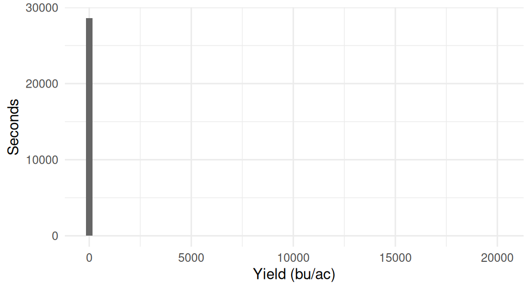
Histogram of yield for every second of the harvest. Everything is pressed into a single bar at the left edge, because the axis has to run out to twenty thousand bushels per acre to fit a handful of readings.
Figure 30.1: Reported yield for every second of the harvest, with no cap.
harvest_agg |>
  filter(yield <= 250) |>
  ggplot(aes(yield)) +
  geom_histogram(bins = 60, fill = "grey40") +
  labs(x = "Yield (bu/ac)", y = "Seconds") +
  theme_minimal(base_size = 11)
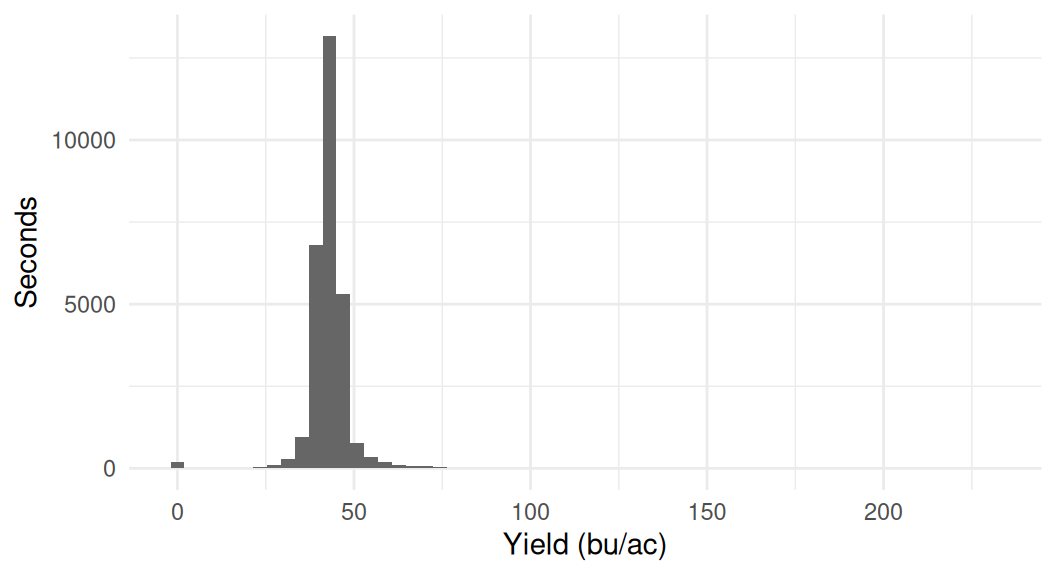
Histogram of yield capped at 250 bushels per acre. A tall symmetric peak sits around forty bushels per acre, with a small bar at zero and a thin tail to the right.
Figure 30.2: The same yields, capped at 250 bu/ac so the shape of the distribution is visible.

We can see in the second histogram that yields are almost all in a believable range, with 96 per cent of seconds between 30 and 55 bu/ac, although there are a handful of zero yields and very large yields that seem implausible. The first histogram makes the extreme yields more visible: the axis has to run out past 20,000 bu/ac to fit them, which squashes everything else into a single bar at the left.

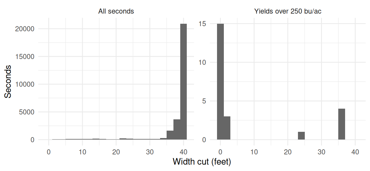
My hunch is that the extreme yields are generally found on the edges of the field. To examine this we can look at the width of the header that is cutting in each second. In the histogram below, the left panel shows the width cut in each second for all seconds, and the right panel shows only the seconds reporting over 250 bu/ac.

For yields that are in a reasonable range, the width cut is almost always the full 40 feet of the header. For the impossible yields, the width cut is often very small – the median is one foot, and not one of them cut more than 39 feet. This suggests some sort of issue around the edges of the field, or when the machine is being turned around.

harvest_agg |>
  mutate(group = ifelse(yield > 250,
                        "Yields over 250 bu/ac",
                        "All seconds")) |>
  ggplot(aes(width_ft)) +
  geom_histogram(binwidth = 2, fill = "grey40") +
  # free_y because 23 seconds and 28,642 cannot share a count axis
  facet_wrap(~group, scales = "free_y") +
  labs(x = "Width cut (feet)", y = "Seconds") +
  theme_minimal(base_size = 11)
Two histograms of the width cut in feet. The left panel, all seconds, has a tall bar at forty feet and a low spread below it. The right panel, impossible yields only, has everything bunched at the far left near zero feet and nothing at forty.
Figure 30.3: Width cut in each second. On the left every second of the harvest; on the right only the seconds reporting over 250 bu/ac.

30.4 Flagging

We could delete these extreme rows now. But I actually want to keep them in so that we could see them on a map in the next chapter. For now let’s put in a flag for yields above 250 bu/ac, yields that are zero, and seconds where less than the full header was cutting, keeping in mind we might want to trim some of these in the future.

harvest_agg <- harvest_agg |>
  mutate(
    # less than the full header was cutting
    flag_partial = width_ft < 39,
    # no grain flow at all
    flag_zero    = yield == 0,
    # no canola crop yields this
    flag_extreme = yield > 250,
    flag_any     = flag_partial | flag_zero | flag_extreme
  )

# across() applies one summary to several columns at once, here every
# column whose name starts with "flag_". A TRUE counts as 1 when summed
harvest_agg |>
  summarise(across(starts_with("flag_"), sum))
> harvest_agg <- harvest_agg |>
+   mutate(
+     # less than the full header was cutting
+     flag_partial = width_ft < 39,
+     # no grain flow at all
+     flag_zero    = yield == 0,
+     # no canola crop yields this
+     flag_extreme = yield > 250,
+     flag_any     = flag_partial | flag_zero | flag_extreme
+   )
> 
> # across() applies one summary to several columns at once, here every
> # column whose name starts with "flag_". A TRUE counts as 1 when summed
> harvest_agg |>
+   summarise(across(starts_with("flag_"), sum))
# A tibble: 1 × 4
  flag_partial flag_zero flag_extreme flag_any
         <int>     <int>        <int>    <int>
1         7720       175           23     7749

30.5 Other checks on the data

Flagging the impossible yields is not the only check worth making. One quick one: yield against the speed the combine was travelling.

harvest_agg |>
  filter(!flag_any) |>
  ggplot(aes(speed_mph, yield)) +
  geom_point(size = 0.3, alpha = 0.05) +
  labs(x = "Speed (mph)", y = "Yield (bu/ac)") +
  theme_minimal(base_size = 11)
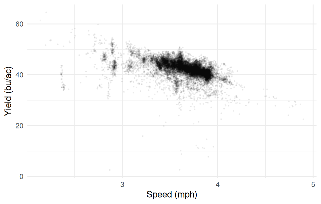
Scatterplot of yield against ground speed. A dense downward-sloping cloud is packed between about 3 and 4 miles per hour, with thin scatter either side of it.
Figure 30.4: Yield against ground speed, for the seconds not flagged above. One point per second, so alpha lets the density show through.

Yield falls as the combine speeds up, and the correlation is -0.50. That is a strong correlation. It could be that we are getting errors when the combine is moving fast. Alternatively, it could be that the operator slows down in heavy crop, in which case the yield is causing the speed rather than the other way round (Section 23.2). Note too that three quarters of the harvest sits between 3.5 and 4.0 mph, so there is very little of the axis to draw a conclusion from.

There are plenty of other checks you could run on a file like this, and which ones are worth your time depends on what you plan to do with the data. Does the moisture reading drift over the day? Do the readings at the start of a pass look different from the ones in the middle? Is the elevation sensible everywhere, or does it jump where the GPS lost its fix? Each is a few lines of the same group_by() and summarise() work, and each tells you something about whether the number you are about to map means what you think it means.

30.6 Field summaries

The number most people want is the field average, and there is more than one way to compute it. We will drop the impossible yields and the zeros first, since neither is a measurement of a crop, but keep the partial cuts.

field <- filter(harvest_agg, !flag_extreme, !flag_zero)

# The simple mean, giving every second the same weight
mean(field$yield)

# Weighted by the width the header was actually cutting
weighted.mean(field$yield, field$width_ft)
> field <- filter(harvest_agg, !flag_extreme, !flag_zero)
> 
> # The simple mean, giving every second the same weight
> mean(field$yield)
[1] 43.53596
> 
> # Weighted by the width the header was actually cutting
> weighted.mean(field$yield, field$width_ft)
[1] 42.83774

The two disagree by about seven tenths of a bushel, and the weighted one is the defensible figure. A second where the header was a quarter in the crop covers a quarter of the ground, so it should count a quarter as much. The simple mean gives it the same say as a full-width second and comes out higher, because those narrow seconds are the ones reading high (Chapter 30).

That gap is a reason to keep the width column rather than a reason to panic: seven tenths of a bushel on forty-three is under two per cent. It would matter more on a field with more edge, and on this one it is the difference between a number you can defend and one you cannot.

One more thing the average does not say. The file covers the ground the combine drove, and the combine drove around two sloughs that take seven and a half acres out of the field’s 139. A yield reported without that gap invites the reader to assume the whole field was measured.

Nothing in the file says the monitor was ever calibrated, and the swath width was typed in by an operator. The only real check on the level would be a weighed total off a scale, and this export does not carry one. Two decimals claim a precision none of that supports, so report 43 bu/ac.

30.7 Exporting the cleaned data

We started with 1.6 million rows and we now have 28,642, one for each second the combine was logging, with the flags attached. That is the version worth keeping: the collapse took a few seconds to run here, but there is no reason to run it again every time we want to look at this field.

##Write the aggregated data out so the next chapter can read it directly
write_csv(harvest_agg, "output/kernen_b1_per_second.csv")
> ##Write the aggregated data out so the next chapter can read it directly
> write_csv(harvest_agg, "output/kernen_b1_per_second.csv")

Writing the result of the slow step, rather than the raw file, is the habit to take away. The script that produced it is the record of how you got there, so anyone – including you in six months – can see which decisions were made and change them.

Chapter 31 picks this up and puts it on a map.