In this chapter, we will create maps from the raw field-level data that we worked with in previous chapters. We will pick up with the file we wrote at the end of Chapter 30, which collapsed the data from a canola field at the University of Saskatchewan’s Kernen farm, east of Saskatoon to one row per second with the flags attached. You can directly download this file here: - kernen_b1_per_second.csv.
We will work with two additional files in this chapter: 1. kernen_b1_boundary.geojson is the field boundary as drawn on the machine’s display, 2. kernen_b1_wetlands.geojson holds the two outlines of two sloughs or wetlands in the field.
31.1 The machine path
The file we are working with is a csv file – not a spatial file. But we can easily convert it to a spatial file by telling R which columns hold the coordinates and what coordinate system they are in. The sf package does this with st_as_sf(), which takes a table and returns a table with a geometry column.
library(tidyverse)library(sf)##Read in the csv fileharvest_agg <-read_csv("data/kernen_b1_per_second.csv", show_col_types =FALSE)# Convert to a spatial objectharvest_sf <-st_as_sf(harvest_agg, coords =c("longitude", "latitude"), crs =4326)## Read the first few rows of this objectharvest_sf
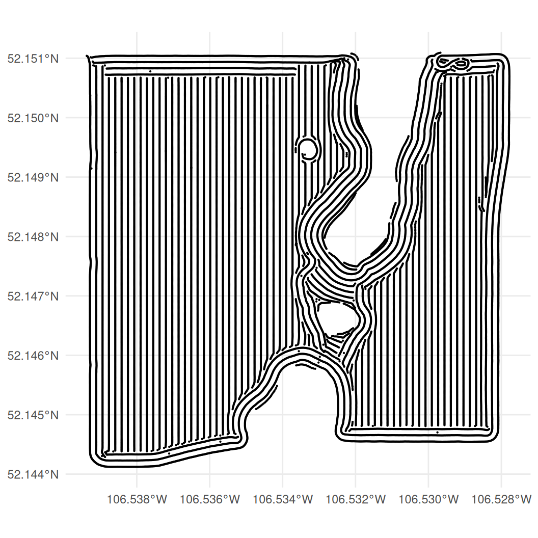
Note that the data in harvest_sf is precisely the same as the data in harvest_agg, except that it has a geometry column. We can now plot the path of the combine through the field using our familiar friends from chapter 6: ggplot() and geom_sf().
ggplot(harvest_sf) +# 28,642 points, so they need to be small to see the patterngeom_sf(size =0.1) +theme_minimal()
Figure 31.1: The combine’s path through B-1. The hole up the middle is a slough, which the machine drove around.
The field is about 810 m across and 780 m top to bottom. Most of it is worked in straight parallel passes, which show as lines of points. However, we see that there are two large spots in the data that have no passes – we will later show that these are sloughs.
31.2 Yield maps
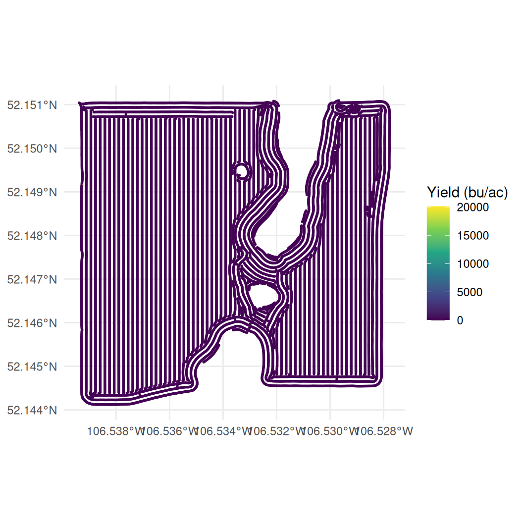
We can make a crude yield map by simply colouring the points according to their yield in the data. Let’s first recall that we still have our crazy yields in the data, so our colour scale is going to be dominated by a handful of these extreme readings.
Figure 31.2: Yield on the raw file. A handful of impossible readings own the colour scale and the field itself is one flat colour.
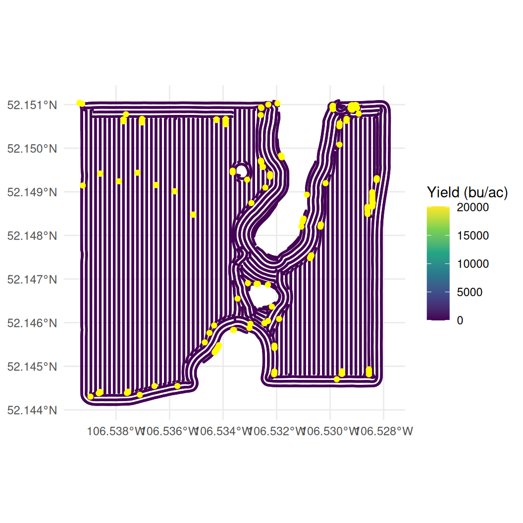
On this map, almost every point is the same dark colour because a handful of impossible readings stretch the colour scale, but there are so few of these observations that we cannot even see them on the map. To make these extreme values more visible, we can create a small data set that contains only the flagged readings. We can then plot these flagged readings on top of the full data set using a large size and a yellow colour.
# A second data set holding only the readings we could not seeflagged <-filter(harvest_sf, flag_extreme | flag_zero)ggplot(harvest_sf) +geom_sf(aes(colour = yield), size =0.3) +scale_colour_viridis_c(name ="Yield (bu/ac)") +labs(x =NULL, y =NULL) +theme_minimal() +# drawn second, so they sit on top of the points belowgeom_sf(data = flagged, colour ="yellow", size =1.5)
Figure 31.3: The same map with the zero and impossible readings picked out in yellow.
There are 198 of these flagged points out of 28,642 – 23 impossible yields and 175 zeros. As expected, most sit near the field boundary, though a handful are scattered through the middle of the field.
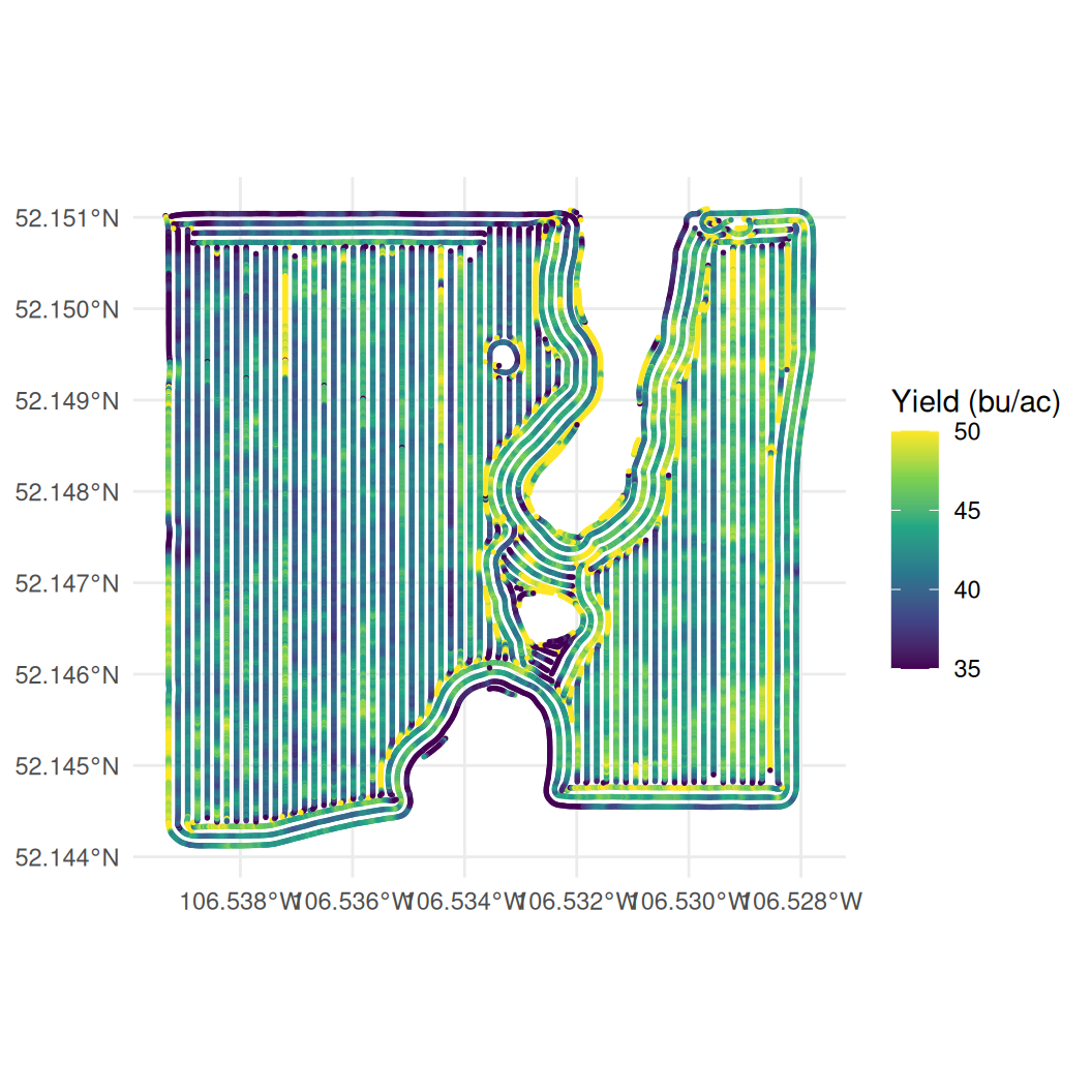
Let’s now remove these extreme value by filtering out the values above 250 bu/acre and the values that are 0 bu/acre.
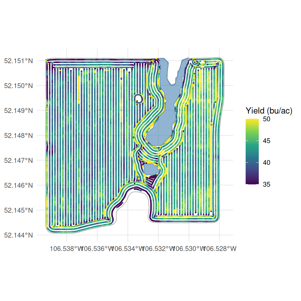
# Drop the readings flagged in the previous chapterclean_sf <-filter(harvest_sf, flag_extreme==FALSE& flag_zero==FALSE)ggplot(clean_sf) +geom_sf(aes(colour = yield), size =0.3) +# squish puts anything outside the limits at the nearest end colourscale_colour_viridis_c(name ="Yield (bu/ac)", limits =c(35, 50),oob = scales::squish) +labs(x =NULL, y =NULL) +theme_minimal()
Figure 31.4: Yield on the cleaned readings.
Now we get a map that shows a bit more variation within the field.
Two things are doing the work here. Dropping the impossible readings helps, but on its own it is not enough: a few readings still run to 231 bu/ac, and one reading that high flattens everything else into a single colour. So the colour scale is fixed to run from 35 to 50 bu/ac, which covers most of the readings, and oob = scales::squish paints anything outside that range in the end colour rather than leaving it blank. The high readings are still on the map, they just stop owning the whole scale. The cost is that the map no longer distinguishes a 50 bu/ac reading from a 231 bu/ac one – both are the brightest colour.
31.3 Merging with the wetland and boundary data
As mentioned, the field has some spots where the combine made no passes. Two visualize these we can use two additional files, one containing the wetlands that are on the field (kernen_b1_wetlands.geojson) and one containing the field boundary (kernen_b1_boundary.geojson).
We can read these files in using st_read() from the sf package, and then layer them on the map we just created.
## Read in boundary and wetlands filesboundary <-st_read("data/kernen_b1_boundary.geojson", quiet =TRUE)wetlands <-st_read("data/kernen_b1_wetlands.geojson", quiet =TRUE)##Add to the mapggplot() +geom_sf(data = boundary, fill =NA, colour ="grey40") +geom_sf(data = clean_sf, aes(colour = yield), size =0.25) +geom_sf(data = wetlands, fill ="steelblue", alpha =0.6,colour ="steelblue4") +scale_colour_viridis_c(name ="Yield (bu/ac)", limits =c(35, 50),oob = scales::squish) +labs(x =NULL, y =NULL) +theme_minimal()
Figure 31.5: The harvested points, the field boundary and the two sloughs.
As expected the boundary file outlines the acrea that was harvested, while the wetlands outline the areas within the fields that were not harvested.
31.4 Aggregating into cells
It is somewhat difficult to see exactly where yields are strongest on the field with the data plotted from the individual readings. This is because individual readings are noisy. A single second of grain flow depends on how full the machine was, whether the driver had just slowed, and where the previous few seconds of crop are in the threshing system. Averaging the readings that fall in the same small area removes most this noise.
This simply involves dividing up the field into cells, and averaging the readings that fall in each cell. The result is a grid of cells with their average yield, which can be plotted as a map.
A grid of cells with a value in each one is a raster, and the terra package handles rasters the way sf handles points and polygons. We do this in two steps:
Build an empty grid of cells over the field with rast(). Cell sizes are given in the units of the coordinate system, so we first project the points to UTM zone 13 north (EPSG 32613), where the units are metres. vect() converts the points from an sf object to the form terra works with.
Use rasterize() to put the readings onto that grid, with fun = mean saying what to do when several readings fall in the same cell.
To see how this works, you can work through the code below step by step to see what is generated on each line.
##Step 1a: change the coordinate system to be expressed in metres rather than degrees of lon and lat, and convert to a terra objectm_pts <-st_transform(clean_sf, 32613) |>vect()##Step 1b: an empty grid of 20 m cells covering the readingsgrid <-rast(m_pts, resolution =20)##Step 2: average the yield of the readings falling in each cellgrid_cells <-rasterize(m_pts, grid, field ="yield", fun = mean)grid_cells
> ##Step 1a: change the coordinate system to be expressed in metres rather than degrees of lon and lat, and convert to a terra object
> m_pts <- st_transform(clean_sf, 32613) |>
+   vect()
>
> ##Step 1b: an empty grid of 20 m cells covering the readings
> grid <- rast(m_pts, resolution = 20)
>
> ##Step 2: average the yield of the readings falling in each cell
> grid_cells <- rasterize(m_pts, grid, field = "yield", fun = mean)
>
> grid_cells
class       : SpatRaster
size        : 39, 40, 1  (nrow, ncol, nlyr)
resolution  : 20, 20  (x, y)
extent      : 394670.9, 395470.9, 5778183, 5778963  (xmin, xmax, ymin, ymax)
coord. ref. : WGS 84 / UTM zone 13N (EPSG:32613)
source(s)   : memory
name        :      mean
min value   : 15.118091
max value   :   147.178
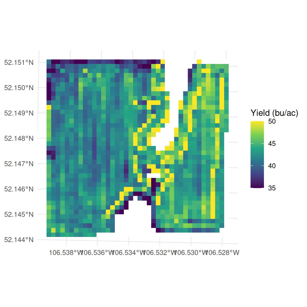
Figure 31.6: Mean yield in 20 m cells. Cells the combine never drove through are empty and show as white.
The resulting map is much easier to read at a glance than the map of individual readings – we can make out areas with higher and lower yields distinctly.
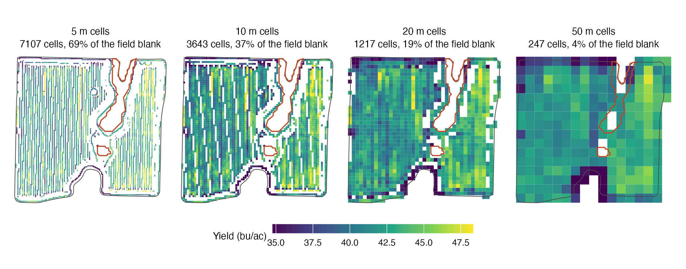
The cells that we used are 20m by 20m, which is a reasonable size for this field. But we could have used any different size by replacing resolution = 20 in the rast() function with a different number. There is an obvious trade-off here: smaller cells keep more detail, but they also have fewer readings in them and are noisier. Larger cells average out the noise, but they also lose detail – it isn’t particularly helpful to just divide the field into two cells and determine whcih one has larger yields. The proper resolution likely depends on your particular application.
Below I illustrate this by creating four maps of the same field, but with different cell sizes. The four maps are all on the same colour scale, so you can see how the colour range changes as the cell size changes.
Figure 31.7: The same readings gridded at four cell sizes, on one colour scale. The slough outlines are drawn on every panel.